Transmission line losses

All transmission lines are characterised by conductivity and dielectric losses. In some cases losses can be neglected, but not in others. When losses are small, some simplifications of transmission line parameters can be made.

The complex propagation constant is $\gamma =\sqrt{(R+\mathrm{jwL})(G+\mathrm{jwC})}$, when the transmission line has low conduction and dielectric losses, we can assume that $R\ll wL$ and $G\ll wC$. Using some mathematical simplifications like the Taylor formula, the propagation constant is $\gamma \approx \mathrm{jw} \sqrt{\mathrm{LC}}(1-\frac{j}{2} (\frac{R}{\mathrm{wL}}+\frac{G}{\mathrm{wC}}).$

So for $y=\alpha +\mathrm{j\beta }, \mathrm{\alpha =}\frac{1}{2} (R \sqrt{\frac{C}{L}}+G\sqrt{\frac{L}{C}}),\mathrm{\beta =}w\sqrt{\mathrm{LC}}$ here $Z_0=\sqrt{\frac{L}{C}}$ is the characteristic impedance. This approximation is called low-loss high frequency approximation and can be used when losses of the transmission line are low.

The formulas we made above appear straight forward. Let’s consider the case of the distortionless transmission line. In general of loss in a transmission line, the propagation constant $\gamma$ will be complicated and the phase term $\beta$ and won’t be a linear function of frequency $w$, so there appears to be phase velocity $v_p=\frac{w}{\beta }$ which will no longer be linear.

It does mean that the different phase parts of the wideband signal will travel with different phase velocities and arrive at the reciever at different times. This effect will lead to the dispersion and the distortion of the signal. So the longer the transmission line, the bigger the phase effect.

The transmission line is distortionless when the parameters are related to the following $\frac{R}{L}=\frac{G}{C}$The propagation constant $\alpha =R\sqrt{\frac{C}{L}}$ and $\beta =w\sqrt{\mathrm{LC}}$. Distortionless transmission lines have losses, but they do not make any distortions.

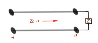
Let’s consider the case of a low-loss transmission line with a certain length $l$ and with $Z_l$ load impedance. Voltage and current for this line are $V\left(z\right)=V_0(e^{–\gamma z}+\Gamma e^{\gamma z}), I\left(z\right)=I_0(e^{–\gamma z}+\Gamma e^{\gamma z})$, where $I_0=\frac{V_0}{Z_0}$.

$\Gamma$ is a reflection coefficient, that depends on the length of the transmission line $Г(l)={\mathrm{Гe}}^{-2\mathrm{\gamma l}}$. The power of the input of the transmission line can be calculated as $\mathrm{Pin}=\frac{1}{2}\mathrm{Re}\left(V\right(–l)I*(-l))$, power on the output of the transmission line is $P_{out}=\frac{1}{2}\mathrm{Re} \left(V_0{I}_0\right)$, so the power losses of the transmission line can be calculated as the difference $P_{loss}=P_{out}–P_{in}$.

Input impedance of the transmission line with length l can be viewed as $Z_{in}=\frac{V(-l)}{I(-l)}$. Power flow across the transmission line helps to find the attenuation constant, and this method is called perturbation method. When the reflections at the transmission line can be estimated as absent, the attenuation constant can be viewed as $\alpha =\frac{P\left(l\right)}{2P(0)}$.

Fields in transmission lines