RF signals – introduction

The radio frequency and microwave field deals with AC signals, with frequencies ranging from 100MHz to 1,000GHz. Radio frequencies usually refer to signals from VHF (30-300MHz) to UHF (300MHz-3,000MHz). The signals in the range 3,000MHz-300GHz are referred to as microwave signals; the signals from 300GHz and higher are referred to as millimetre signals.

The RF and microwave theory can not use standard circuit theory, because of high frequencies and small wavelengths. Here, standard circuit theory is an approximation. Current and voltage phase change significantly across the devices with high frequencies. In contrary for small frequencies (with big wavelength), signal phase does not change very much along the device. That is why microwave components can behave like distributed components. From the other side, the wavelength of the signal is much shorter than the device, and the system can be designed from the point of view of geometrical optics. And the system can be called quasi-optical. The Table 1 shows frequency bands gradation.

The applications of microwave and RF signals surrounding us in our daily life, and RF signals are the basis for the communications area. The cellular signals, known as 2G, 3G, 4G are based on the different schemes of signal modulation and more modern types of data transmission.

RF signalling is also used in the other wireless communication systems like sensing. Satelite technologies are based on RF and MW signalling, and have been designed to transmit cellular signals all over the world. The Global Positioning System (GPS) and Wireless Local Area Networks (WLAN) work successfully due to RF and MW signalling.

Radar systems, based on RF and MW technologies, have applications in different areas – civil, military, and research. Military radars are designed to detect targets in the sea, on the ground or in the air; civil radars work in transport surveillance systems, airport landing and departing systems and metro stations; research radars are used for scientific purposes. Microwave radiometry is used for monitoring the atmosphere, in medical investigations and for security purposes.

BAND FUNCTION	FREQUENCY RANGE
AM broadcast band	525-1705kHz
Shortwave radio	3-30 MHz
WHF TV	54-72, 76-88, 174-216 MHz
FM broadcast band	87.8-108 MHz
Aircraft radio	108-136 MHz
Commercial and public safety	150-174 MHz
UHF TV	470-806 MHz
Wireless	698-806 MHz, 1.71-1.78, 1.8-1.91, 1.93-1.99 GHz
Public safety	806-940 MHz
Cell phones	824-849, 869-894, 876-960 MHz
L-band (IEEE)	1-2 GHz
S-band (IEEE)	2-4 GHz
C-band (IEEE)	4-8 GHz
Microwave ovens	2.45 GHz
X-band (IEEE)	8-12 GHz
Ku-band (IEEE)	12-18 GHz
K-band (IEEE)	18-26 GHz
Ka-band (IEEE)	26-40 GHz
V-band (IEEE)	40-75 GHz
W-band (IEEE)	75-110 GHz
Millimeter-wave	110-300 GHz

Table 1. Frequency bands according to different defining organisations IEEE, EU, NATO.

 RF and microwave started since 19th century when James Clerk Maxwell proved electromagnetic waves propagation mathematically, and showed that light is an electromagnetic wave. Oliver Heaviside designed the mathematical language that all engineers understand.

He also provided the base for guided-wave and transmission line theories. Heinrich Herz verified Maxwell’s theory with some experiments. He also demonstrated first reflector antennas, velocity of electromagnetic wave propagation, and other RF techniques.

Another important investigation was metal wave-guides by Southworth at AT&T and Barrow at MIT. Magnetron and klystron were invented slightly before the Second World War. The first radar was built in Great Britain, and was developed in the US and Germany simultaneously. At the beginning of 1950s microstrip transmission lines were developed, which became the basis for the modern planar technology in microelectronics.

Magnetrons, klystrons, travelling wave tubes and other devices were pretty big and required additional equipment to operate. So scientists continued the development towards smaller devices. The first MW GaAs MESFET was made in 1955 at CalTech. It was the beginning of the era of Monolitic Microwave Integrated Circuits, where the transmission lines are based on the semiconductor substrate together with active devices.

The overview of electromagnetic theory can be seen in our module chapter Electromagnetic waves and fields. So here we only touch the main points as a refresher. RF and MW theory is very strongly based on planar waves propagation. The planar wave is the simplest of electromagnetic waves. Maxwell’s equation looks like this:

$$\begin{gathered} \nabla E=\frac{\partial B}{\partial t}–M; \\ \nabla H=\frac{\partial D}{\partial t}+J; \\ \nabla D=\rho ; \\ \nabla B=0; \end{gathered}$$

The source of the elelctromagnetic field are currents M and J. For the vacuum the following relations between elelctric and magnetic fields are valid:

$$\begin{gathered} B={\mu }_{0}H,D={\epsilon }_{0}E; \\ {\mu }_0=4\pi *\frac{{10}^{–7}Hn}{m}; {\epsilon }_0=8.854*{10}^{–12}F/m. \end{gathered}$$

${\mu }_0$ and ${\epsilon }_0$ are permeability and permittivity of a vacuum.

The integral form of the equations above are:

$$\begin{gathered} {\oint }_s Dds={\int }_v^{}\rho dv=Q; \\ {\oint }_s Bds=0; \\ {\oint }_c Edl=–\frac{\partial }{\partial t}{\int }_{s}Bds–{\int }_{s}Mds; \\ {\oint }_c Hdl=\frac{\partial }{\partial t}{\int }_{s}Dds+{\int }_{s}Jds=\frac{\partial }{\partial t}{\int }_{s}Dds+I \end{gathered}$$

As far as the involved fields are harmonical, then E(r,t) = E(r,t) cos(ωt + φ) e_r, E(r) = A(r)e^j(ωt+φ)e_r. Assuming these field are time dependent and apply them to the Maxwell equations:

$$\begin{gathered} \left[\nabla ,E\right]=–j\omega B–M; \\ \left[\nabla ,H\right]=j\omega D+J; \\ \nabla D=\rho ; \\ \nabla B=0 \end{gathered}$$

The formulas above are assumed in the vacuum. Electromagnetic fields exist in materials too and they are related in a special way. An electric field causes polarisation of the atoms and molecules, so total displacement flux will be:

$D={\epsilon }_{0}E+{\epsilon }_0{X}_{e}E=\epsilon 0E+P_e={\epsilon }_0(1+X_e)E$

$P_e$ is an electric polarisation, $X_e$ is an electric susceptibility.

$D=\epsilon E, where \epsilon ={\epsilon }_0(1+X_e)=\epsilon ‘–j\epsilon “$

is a complex permittivity of the matter. The imaginary part of the permittivity is related to losses. For anisotropic materials electric field is a tensor quantity.

$\left[\begin{array}{c}{D}_x\\ D_y\\ D_z\end{array}\right]=\left[\begin{array}{c}{\epsilon }_{xx}{\epsilon }_{xy}{\epsilon }_{xz}\\ {\epsilon }_{yx}{\epsilon }_{yy}{\epsilon }_{yz}\\ {\epsilon }_{zx}{\epsilon }_{zy}{\epsilon }_{zz}\end{array}\right]\left[\begin{array}{c}{E}_x\\ E_y\\ E_z\end{array}\right]=\left[\epsilon \right]\left[\begin{array}{c}{E}_x\\ E_y\\ E_z\end{array}\right]$

Magnetic fields can effect dipoles of the molecules and atoms too, producing magnetic polarisation P_m, and B = (H + P_m) µ₀ = µ₀(1 + X_m) H = µH, where µ = µ₀ (1 + X_m) = µ’ – jµ” is magnetic susceptibility. It’s imaginary part is also related to losses. For anisotropic magnetic materials (for example ferrimagnetics) the magnetic field is a tensor quantity:

$\left[\begin{array}{c}{B}_x\\ B_y\\ B_z\end{array}\right]=\left[\begin{array}{c}{\mu }_{xx}{\mu }_{xy}{\mu }_{xz}\\ {\mu }_{yx}{\mu }_{yy}{\mu }_{yz}\\ {\mu }_{zx}{\mu }_{zy}{\mu }_{zz}\end{array}\right]\left[\begin{array}{c}{H}_x\\ H_y\\ H_z\end{array}\right]=\left[\mu \right]\left[\begin{array}{c}{H}_x\\ H_y\\ H_z\end{array}\right]$

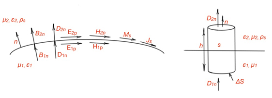
Let’s consider the interface between two materials (Figure 1). Maxwell’s equation:

${\oint }_s Dds={\int }_v\rho dv goes to D_{2n}∆S–D_{1n}∆S=∆S=∆S{\rho }_s, so (D_2–D_1)n={\rho }_s$

ρ_s is a charge density on the interface between two matters. For magnetic fields B₁n = B₂n. For the Maxwell equation:

${\oint }_c Edl=–\frac{\partial }{\partial t}{\int }_{s}Bds–{\int }_{s}Mds will be E_{1\rho }∆l–E_{2\rho }∆l=–Ms∆, then (E_2–E_1)n=M_s$

For the magnetic field (H₂ – H₁) n=J_s, here J_s is an electric current on the surface, n is a normal vector. These relations are valid for all interfaces between general matters.

Let’s consider lossless dielectric interfaces. For this interface (there is no charge between them) the following relations will work:

$\begin{array}{c}n{D}_1=n{D}_2;\\ n{B}_1=n{B}_2;\\ n{E}_1=n{E}_2;\\ n{H}_1=n{H}_2\end{array}$

For the interface where one of the matters is a good conductor (metal), this condition always leads to different circumstances in RF engineering. All the field components should be 0 in the metal, conductivity is σ → ∞, then: σ →

$\left[\begin{array}{c}nD={\rho }_s;\\ nB=0;\\ nE=0;\\ nH=J_s\end{array}\right]$

This interface is known as an electric wall – here ρ_s and J_s are charge and current densities, the normal vector n points out of the metal.

An interface with a good magnetic material is known as a magnetic wall  – the boundary conditions will be:

$\left[\begin{array}{c}nD=0;\\ nB=0;\\ nE=–M_s;\\ nH=0\end{array}\right]$

The normal vector n is pointing out the magnetic material.

Let’s consider linear, isotropic and homogeneous matter. The Maxwell equations will be:

$\left\{\begin{array}{l}[\nabla ,E]=–j\omega \mu H\\ [\nabla ,H]=j\omega \epsilon E\end{array}\right.$

Let’s resolve this system of equations, expressing one quantity through another. From mathematics we know that:

$[\nabla ,[\nabla ,X\left]\right]=(\nabla ,(\nabla ,X\left)\right)–{\nabla }^{2}X. Then {\nabla }^{2}E+{\omega }^2\mu \epsilon E=0 and {\nabla }^{2}H+{\omega }^2\mu \epsilon H=0.$

The constant $\omega \sqrt{\mu \epsilon }$ is called the propagation constant and the equations for vectors $E$ and $H$ are Helmholz equations.

For the lossless matter µ  and ɛ are the real numbers. Let’s consider the elelctric field E with only the x component distributing in the uniform (x, y)  plane. Then the Helmholtz equation will be the following:

$\frac{{\partial }^2{E}_x}{\partial z^2}+{\omega }^2\mu \epsilon E_x=0$

Assuming that ω²µɛ = α² is a constant, the solution of this equation is:

$E_x\left(z\right)=E^{+}{e}^{–jaz}; E(z,t)=E^{+}\cos (\omega t–\alpha z)+E^{–}\cos (\omega t+\alpha z)$

This is the wave representation of the electric field, and as you can see it has positive and negative movement directions. The phase velocity of the wave is:

$v_{\rho }=\frac{\omega }{\alpha }=\frac{1}{\sqrt{\mu \epsilon }}$

For the vacuum it is 2.998 * 10⁸m/sec. The wavelength is:

$\lambda =\frac{2\pi }{\alpha }$

The electromagnetic field will also have the magnetic component:

$H_y=\frac{j}{\omega \mu }\frac{\partial E_x}{\partial z}=\sqrt{\frac{\epsilon }{\mu }(E^{+}{e}^{–jaz}+}{E}^{–}{e}^{jaz})$

The constant $\sqrt{\frac{\epsilon }{\mu }}$is called intrinsic impedance of the matter. The intrinsic impedance of free space is $\sqrt{\frac{{\mu }_0}{{\epsilon }_0}}=3.77 Ohm$.

The H and E are orthogonal to each other and to the propagation direction, transverse electromagnetic waves (TEM).

Let’s consider matter with losses, it should be conductive matter. And the Maxwell equations in this case are:

The wave equation is $\nabla 2E+\omega 2\mu \epsilon (1–j\frac{\delta }{\omega \epsilon })=0$. The propagation constant is complex $$\begin{gathered} \left[\begin{array}{cc}\nabla ,& E\end{array}\right]=–j\omega \mu H \\ \left[\begin{array}{cc}\nabla ,& H\end{array}\right]=j\omega \epsilon E+\delta E \end{gathered}$$ and $\gamma =\alpha +\beta i=j\omega \sqrt{\mu \epsilon (1–j\frac{\delta }{\omega \epsilon })}$ , $\alpha$ is an attenuation constant, $\beta$ is a phase constant. The intrinsic impedance is complex $\frac{j\omega \mu }{\gamma }$.

Let’s consider a good conductor; here the actual conductive current is greater than the displacement current, and it means σ >> ωɛ, so we can ignore the displacement current in the propagation current:

$\gamma =j\omega \sqrt{\mu \frac{\delta }{j\phi \epsilon }} =(1+j)\sqrt{\frac{\omega \mu \delta }{2}}$

Here we can define the skin depth, and the parameter characterising field penetration depth:

${\delta }_s=\sqrt{\frac{2}{\omega \mu \delta }.}$ The intrinsic impedance is $(1+j)\frac{1}{\delta {\delta }_S}$.

Let’s consider the plane waves and discover their general features. The Helmholtz equation for a vacuum is:

$$\begin{gathered} \nabla 2E+{\alpha }_0^{2}E=\frac{{\partial }^{2}E}{\partial x^2}+\frac{{\partial }^{2}E}{\partial y^2}+\frac{{\partial }^{2}E}{\partial z^2}+{\alpha }_0^{2}E–0; \\ and \frac{{\partial }^2{E}_i}{\partial x^2}+\frac{{\partial }^2{E}_i}{\partial y^2}+\frac{{\partial }^2{E}_i}{\partial z^2}+{\alpha }_0^2{E}_i=0 \end{gathered}$$

Here we use the variables separation method, where we assume E_x(x,y,z) = f(x)g(y)h(z). The Helmholtz equation with this assumption is the following:

$$\begin{gathered} \frac{f“}{f}+\frac{g“}{g}+\frac{h“}{h}+{\alpha }^2=0, \\ \frac{{\partial }^{2}f}{\partial x^2}+{\alpha }_x^{2}f=0,\frac{{\partial }^{2}g}{\partial y^2}+{\alpha }_y^{2}g=0,\frac{{\displaystyle {\partial }^{2}h}}{{\displaystyle \partial z^2}}+{\alpha }_z^{2}h=0; {\alpha }_x^2+{\alpha }_y^2+{\alpha }_z^2={\alpha }^2 \end{gathered}$$

The solution for the equations is:

$\begin{array}{c}{E}_x(x,y,z)=A{e}^{–jkr};\\ E_y(x,y,z)=B{e}^{–jkr};\\ E_z(x,y,z)=C{e}^{–jkr}\end{array}$ $Then E=E_0{e}^{–jar}).(\nabla ,E)=0$. Here $r$ and $k$ are vectors.

$0$ means that the electric field is orthogonal to the propagation direction. The Maxwell equation states:

$[\nabla ,E]=–j\omega \mu H, so H=\frac{{\alpha }_0}{\omega {\mu }_0}[n,E]=\frac{1}{{\eta }_0}[n,E],$

where n is a vector normal to the interface and η₀ is the intrinsic impedance of the vacuum. The time variable expression for an electric field is:

$E(x,y,z,t)=Re\left\{E\right(x,y,z\left)e^{j\omega t}\right\}=E_0\cos (ar–\omega t)$

We have considered linearly polarised  waves above. However, the waves can be also circularly polarised, left-hand circularly polarised and right-hand circularly polarised. The right-hand circularly polarised wave is when the fingers are pointing the E rotation and the thumb finger points in the direction of propagation. For left-hand circularly polarised waves the electric field rotates in the opposite direction. Magnetic field here can be found from one of Maxwell’s equations, and it will correspond to the direction of the electric field rotation. It means right-hand polarised electric fields correspond to the right-hand polarised magnetic field.

The source of electromagnetic energy carries the power that can be transmitted or dissipated. In a general case deriving and integrating Maxwell equations, we will get the Poynting theorem statement. The complex power P_s enclosed in the surface S, is delivered by the J_s and M_s flows is:

$P_s=–\frac{1}{2}{\int }_v(EJ{*}_s+H*M_s)dv$

Let’s consider the Poynting vector $S=\left[E,H^{*}\right]$, and power is $P_0=\frac{1}{2}{\oint }_S\left[E,H^{*}\right]dS=\frac{1}{2}{\oint }_{S}SdS$.

So the power of the electromagnetic source enclosed in the value V is the following (you can do Maxwell’s equations derivation and integration by yourself, or check the resources in the preface to the RF and Microwave chapter):

$P=\frac{\delta }{2}{\int }_v|E{|}^{2}dv+\frac{\omega }{2}{\int }_v (\epsilon “|E{|}^2+\mu “|H{|}^2)dv,$ that is Joule’s Law.

So the complex power, according to the Poynting theorem is P_s = P0 + P + 2jω(W_m-W_e), which represents the power transmitted through the surface, power spent to heat and 2ω reactive energy in the volume V.

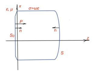
Let’s consider a good conductor. The real transmission line containing practical conductors is characterised by attenuation, power losses and noise generation. To calculate these characteristics we must calculate the power dissipation of the conductor. Figure 2 shows the interface between the lossless matter and a practical conductor.

The power through the conductor through the S and S0 is: $P=\frac{1}{2}Re{\int }_{S+S_0}\left(\right[E,H*],n)dS$.

Proper selection of the surface S can make the: ${\int }_S\left(\right[E,H*],n)dS=0$.

So we are considering the average power through the surface S0:

$P=\frac{1}{2}Re{\int }_{S_0}\left(\right[E,H*],z)dS$

From the mathematics we know that (z,[E,H*]) = (H*,[E,z]) = η(H*,H), so:

$P=\frac{R_S}{2}{\int }_{S_0}|H{|}^{2}ds,R_s=Re=Re\{\eta \}=\frac{1}{\delta {\delta }_S}, where R_S is called the surface resis\tan ce of the conductor.$

Plane electromagnetic waves can also reflect from the interfaces with different matters. Let’s consider the interface between lossless matter and a practical conductor. The electromagnetic wave, going from the side of the lossless matter, is:

$E_p=E_0{e}^{–jaz}x,H_p=\frac{1}{\eta 0}{E}_0{e}^{–jaz}y$

P index states that these waves are propagating waves. η₀ is the impedance of the vacuum, E₀ is the wave magnitude. The reflected waves have the form:

$E_r=E_0Гe^{jaz}x,H_p=–\frac{Г}{{\eta }_0}{E}_0{e}^{jaz}y$

Where Г is a reflection coefficient of the reflected electromagnet wave.

In the loss material the electromagnetic wave will look like the following:

$E_l=x{E}_{0}L{e}^{–yz},H_{l}y\frac{L{E}_0}{\eta }{e}^{–yz}$

L is the transmission coefficient in the loss material, the ‘l’ index means here is the loss-environment. The η is an intrinsic impedance as we’ve learned above. Now we have four equations for E and H and two unknown Г and L.

When applying the boundary condition z=0, fields should be continuous here, and we can get a solution for the reflection and transmission coefficient.

$Г=\frac{\eta –{\eta }_0}{\eta +{\eta }_0,}L=\frac{2\eta }{\eta +{\eta }_0}$

These formulas represent the general case of the reflection and transmission of the normally incidental waves.

Let’s consider several cases of the material interacting with lossless matter. If the second material is the lossless matter, then ,  and  are the real numbers. The propagation constant is:

$$\begin{gathered} \gamma =j\beta =j\alpha \sqrt{{\mu }_r{\epsilon }_r,} \alpha =\omega \sqrt{{\mu }_0{\epsilon }_0} \\ The wavelength is \lambda =\frac{2\mathrm{\pi }}{\omega \sqrt{\mu \epsilon }}, \\ intrinsic impedance is \eta =\sqrt{\frac{\mu }{\epsilon }}, phase velocity v_p=\frac{1}{\sqrt{\mu \epsilon }} \end{gathered}$$

Poynting vectors for both matters are:

$S^{+}=z\left|E_0{|}^2\frac{1}{{\eta }_0}\right(1–\left|Г{|}^2\right), S^{–}=z\left|E_0{|}^2\right(1–|Г{|}^2+2jГ\sin 2\alpha z)$

At the interface between two materials S⁺ = S^–. The average power for two regions is:

$P^{+}=\frac{1}{2}\left|E_0{|}^2\frac{1}{{\eta }_0}\right(1–\left|Г{|}^2\right), P–=\frac{1}{2}\left|E_0{|}^2\frac{1}{{\eta }_0}\right(1–\left|Г{|}^2\right)$

Then we see that power is conserved S⁺ = S^–.

For the good conductor the constants become complex.

$$\begin{gathered} The propagation cons\tan t \gamma =\alpha +j\beta ==(1+j) \frac{1}{{\delta }_S}, \\ the intrinsic impedance \eta =(1+j)\frac{1}{\delta {\delta }_S}, \\ and as it is complex vectors E and H are shifted to \frac{\mathrm{\pi }}{4}. \\ Skin depth {\delta }_S=\frac{1}{\alpha }. \end{gathered}$$

Considering Poynting vectors:

$S^{+}=z\left|E_0{|}^2\frac{1}{{\eta }_0}\right(1–|Г{|}^2+Г–Г*)e^{–2\alpha z},S^{–}=z\left|E_0{|}^2\frac{1}{{\eta }_0}\right(1–{|}^2+Г–Г*)$

At the interface S⁺ = S^–. The electric volume current density flowing through the conductor is:

$J_l=\delta E_l=x\delta E_{0}L{e}^{–yz}$

The average power dissipating through the volume of semiconductor is:

$P_l=\frac{\delta \left|E_0{|}^2\right|L{|}^2}{4\alpha }$

Surface impedance is very important for analysis of plane electromagnetic waves transmission through the materials, and the wave transmission through the  imperfect material. When the plane electromagnetic wave occurs on the interface with a good conductor, part of it usually reflects and part of it transmits with losses, decreasing in a very thin layer close to the surface of a conductor. Using the formulas and laws shown above, like Joule’s Law, and the current flow calculation of the Poynting theorem, we get the same result for power dissipating in the conductor:

$P_l=2(\frac{E^0}{{\eta }_0}{)}^2{R}_S, R_S=Re\{\eta \}=\sqrt{\frac{\omega \mu }{2\delta }}$

All the parameters mentioned above are the parameters of matter or electromagnetic wave.

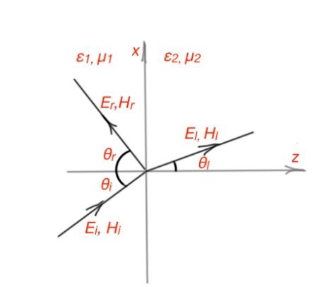
Before we consider the normal incidents of an electromagnetic wave, we will consider the oblique incidence of electromagnetic waves (Figure 3. In this case the electromagnetic waves will polarise – parallel or perpendicular way). For parallel polarisation the electric field wave is in the XZ plane and the incident looks like this:

$$\begin{gathered} E_i=E_0(x\cos {\theta }_i–z\sin \theta i)e^{–j\alpha 1(x\sin {\theta }_i+z\cos \theta i)}, H_i=y \frac{E_0}{{\eta }_0}{e^{–j{\alpha }_1}}^{(x\sin {\theta }_i+z\cos {\theta }_i)}, \\ where {\alpha }_1=\omega \sqrt{{\mu }_0{\epsilon }_1,{\eta }_1}=\sqrt{\frac{{\mu }_0}{{\epsilon }_1}}is the propagation cons\tan t and surface impedance of region 1. \end{gathered}$$

For the reflected and transmitted waves we have:

$$\begin{gathered} E_r=E_0Г(x\cos {\theta }_r+z\sin {\theta }_r)e^{–j{a}_1(x\sin {\theta }_r–z\cos \theta r)},H_r=–\frac{E_0}{{\eta }_1}Гy{e}^{–j{a}_1(x\sin {\theta }_r–z\cos \theta r)}, \\ {E}_l=E_{0}L(x\cos {\theta }_l–z\sin {\theta }_l{)}^{e–j{a}_2(x\sin {\theta }_l+z\cos {\theta }_l)},H_l=\frac{E_0}{{\eta }_2}Гy{e}^{–j{a}_2(x\sin {\theta }_l+z\cos {\theta }_l)} \end{gathered}$$

The corresponding coefficients and constants here are:

${\alpha }_2=\omega \sqrt{{\mu }_0{\epsilon }_2,{\eta }_2}=\sqrt{\frac{{\mu }_0}{{\epsilon }_2}}$

Here we have four equations for four unknowns:

${\theta }_l,{\theta }_r,Г,L$

Resolving this system, we get Snell’s Law: Ɵ_i = Ɵ_r, a₁sinƟ_i = a₂sinƟ_l. The reflection and transmission coefficients are:

$Г=\frac{{\eta }_2\cos {\theta }_l–{\eta }_1\cos {\theta }_i}{{\eta }_2\cos {\theta }_l+{\eta }_1\cos {\theta }_i}, L=\frac{2{\eta }_2\cos {\theta }_i}{{\eta }_2\cos {\theta }_l+{\eta }_1\cos {\theta }_i}$

From here we can find the Brewster angle when:

$Г=0: \sin {\theta }_b=\frac{1}{\sqrt{1+{\displaystyle \frac{\epsilon 1}{\epsilon 2}}}}. And \cos {\theta }_l=\sqrt{1–\frac{{\alpha }_1^2}{{\alpha }_2^1}} {\sin }^2{\theta }_b,$

The propagation constants α₁, α₂ are known from the paragraph above.

Also possible is perpendicular polarisation. In this case the electromagnetic wave is perpendicular to XZ plane. The incident wave is:

$H_i=\frac{E_0}{{\eta }_1}(–x\cos {\theta }_i+z\sin {\theta }_i)e^{–j{a}_1(x\sin {\theta }_i+z\cos {\theta }_i)},E_i=y{E}_0{e}^{–j{a}_1(x\sin {\theta }_i+z\cos {\theta }_i)},$

where the propagation constant and internal impedance are:

$\alpha 1=\omega \sqrt{{\mu }_0{\epsilon }_1,}{\eta }_1=\sqrt{\frac{{\mu }_0}{{\epsilon }_1}}$

Transmission Line Theory