Fourier function representation

This post covers topic of fourier representation of a function. Most signals are represented with a set of exponential functions, resulting in complex exponential functions. If these functions are affected with exponential external impact, the resulting function will be exponential, but with different amplitude $\left\{\begin{array}{l}{e}^{st}\to H\left(s\right)e^{st}\\ z^n\to H\left(z\right)z^n\end{array}\right.$ . $H\left(s\right)$ and $H\left(z\right)$ can be complex functions as well.

These functions are eigenfunctions and the amplitudes are eigenvalues. It can be easily shown that for discrete and continuous time functions, if the input function is represented with a complex exponential function, the resulting function will be a linear combination of complex exponential functions. Here, exponential functions will be eigenfunctions and coefficients – eigenvalues.

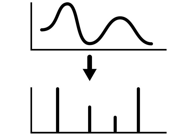
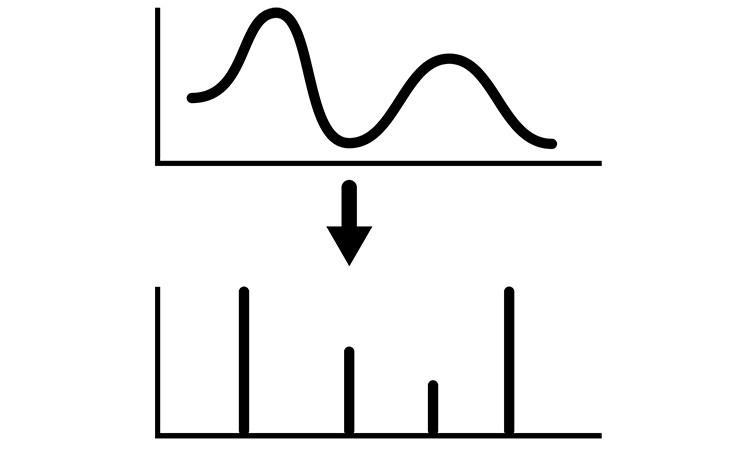
As we know, the continuous time function $f\left(t\right)=f(t+T)$ is a periodic function where T is a fundamental period, $w_0=\frac{2\mathrm{\pi }}{T}$ is a fundamental frequency. The function $f\left(t\right)=\sum _{k=–\infty }^{\infty }{C}_k{e}^{j{w}_{0}t}$ is also a periodic function with a fundamental period $T$. This representation of a periodic signal is called Fourier series representation. Let’s consider some statements of Fourier signals.

1. Assume that periodic continuous –time function $f\left(t\right)$ can be described with the Fourier series $f\left(t\right)=\sum _{n=–\infty }^{\infty }{C}_n{e}^{j{w}_{0}t}$, so $f^{*}\left(t\right)=f\left(t\right)$. We can see that $f^{*}\left(t\right)={\int }_{n=–\infty }^{+\infty }{C_{–n}}^{*}{e}^{–j{w}_{0}t}, {C_{–n}}^{*}=C_n$.
2. The Fourier series $f\left(t\right)=\sum _{n=–\infty }^{\infty }{C}_n{e}^{j{w}_{0}t}$ can also be represented in its trigonometric forms $f\left(t\right)=c_0+2\sum _{n=1}^{+\infty }{C}_n\cos (n{w}_{0}t+\phi )$ and $f\left(t\right)=a+2\sum _{n=1}^{+\infty }(b_n\cos n{w}_{0}t–c_n\sin n{w}_{0}t)$. Both of the last expressions can be represented one from another. The trigonometric function representation goes from the exponential function representation. So you can easily show that these expressions go from one to the other.

Let’s consider time-continuous periodic function $x\left(t\right)$ with a fundamental period $t=T$ and fundamental frequency $w_0=\frac{2\mathrm{\pi }}{T}$. So, the Fourier series representation of this function can be described as: $f\left(t\right)=\sum _{n=–\infty }^{\infty }{C}_n{e}^{jn\frac{2\mathrm{\pi }}{T}t}, C_n=\frac{1}{T}{\int }_{T}f\left(t\right)e^{–\frac{2\mathrm{\pi }}{T}}tdt$. Here the coefficients $C_n$ are Fourier coefficients.

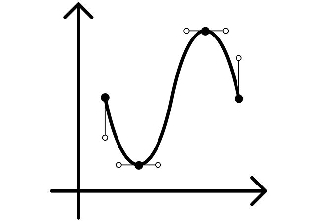
The Dirichlet conditions guarantee that its Fourier function $x\left(t\right)$ is equal to its Fourier representation, except some t intervals where it is discontinued. On these intervals function has the average value.

Dirichlet condition I. ${\int }_T\left|f\left(t\right)\right|dt<\infty ,$ and $\left|C_n\right|<\infty$ Dirichlet condition II. During a finite period of time, the function $f\left(t\right)$ is limited with its minimum and maximum values.
Dirichlet condition III. In any finite interval there is a finite number of discontinuities. Every discontinuity is finite.

You can easily check the Fourier representation of every periodic function without discontinuities at the interval $–t$ is equal to the initial function. Every periodic function with a finite amount of discontinuities on the interval, t is equal to the initial function, except some points that are the average value of a function.

If the function is identical to its Fourier representation, except for some points, then we can assume that the signals behave identically under convolution and we can expect them to be identical during LTI system analysis.

Let’s consider the properties of Fourier series functions. Let’s consider periodic function $f\left(t\right)$ with the period $T$, and its Fourier coefficients $a_n$, so we can assign them together $f\left(t\right)\leftrightarrow c_n$.

1. Linearity property. If the functions $f\left(t\right)$ and $g\left(t\right)$, are periodic with period $T$, with Fourier coefficients $f\left(t\right)\leftrightarrow c_n$, $g\left(t\right)\leftrightarrow b_n$ then the Fourier coefficients for function $z$.
2. $h\left(t\right)=Af\left(t\right)+Bg\left(t\right)$ are $h\left(t\right)=A{c}_n+B{b}_n$.
3. Time shift. If the function $f\left(t\right)$ is periodic with period $T$, then the Fourier representation for a time shifted signal $g\left(t\right)=f(t–t_0)$ is characterised with coefficients $g\left(t\right)\leftrightarrow c_n{e}^{–jn\frac{2\mathrm{\pi }}{T}{t}_0}$.
4. Time reversing. If the function $f\left(t\right)$ is periodic with period $T$, and has the Fourier representation $f\left(t\right)\leftrightarrow c_n$, then the reversed function has the following Fourier representation $f(–t)\leftrightarrow –c_n$, if $f\left(t\right)$ is odd, and $f(–t)\leftrightarrow c_n$, if $f\left(t\right)$ is even.
5. Time scaling. If the periodic function $f\left(t\right)$ has a period T and is characterised with Fourier representation $f\left(t\right)\leftrightarrow c_n$, then the periodic function $f\left(kt\right)$, where $k$ is a real number we have the period $\frac{T}{k}$ with the Fourier representation $f\left(kt\right)=\sum _n^{}{c}_n{e}^{–jnk{w}_{0}t}$. Here $f\left(kt\right)\leftrightarrow c_n$, but the period and frequency will be scaled in accordance with the scaling coefficient.
6. Multiplication. If the functions $f\left(t\right)$ and $g\left(t\right)$ are periodic functions with period $T$ and Fourier representations $f\left(t\right)\leftrightarrow c_n$, $g\left(t\right)\leftrightarrow b_n$, then multiplication $f\left(t\right)g\left(t\right)$ will be characterised with Fourier coefficients $d_n=\sum _{k=–\infty }^{\infty }{c}_k{b}_{n–k}$.
7. Conjugation. For the periodic function $f\left(t\right)$ with period $T$, characterised with Fourier representation $f\left(t\right)\leftrightarrow c$, then for conjugated function $f^{*}\left(t\right)$ will have the Fourier representation $f^{*}\left(t\right)\leftrightarrow {c_{–k}}^{*}$.
8. Parseval’s relation. For the periodic function $f\left(t\right)$ with Fourier representation $f\left(t\right)\leftrightarrow c_n$ the Parseval relation is valid $\frac{1}{T}{\int }_T{\left|f\left(t\right)\right|}^{2}dt=\sum _{n=–\infty }^{\infty }{\left|c_n\right|}^2$ .

Let’s consider a descrete time periodic signal $f\left[n\right]=f\left[n+N\right]$, where $N$ is the period of the descrete time function. This function can be presented in an exponential form $f\left[n\right]=\sum _n^{}{c}_n{e}^{j\frac{2\mathrm{\pi }}{N}n}$. So this function can be characterised with the following Fourier representation $f\left[n\right]=\sum _l{c}_l{e}^{j\frac{2\mathrm{\pi }}{N}n}$, where $c_l=\frac{1}{N}\underset{n}{\sum f\left[n\right]}{e}^{–jl\frac{2\mathrm{\pi }}{N}n}$ . Here below are properties of a Fourier series for descrete-time periodic signals:

1. Linearity property. If the functions $f\left[n\right]$ and $g\left[n\right]$, are periodic with period $N$, with Fourier coefficients $f\left[n\right]$$\leftrightarrow c_n$, $g\left[n\right]\leftrightarrow b_n$ then the Fourier coefficients for function $h\left[n\right]=Af\left[n\right]+Bg\left[n\right]$ are $h\left[n\right]\leftrightarrow A{c}_n+B{b}_n$.
2. Time shift. If the function $f\left[n\right]$ is periodic with period $N$, then the Fourier representation for a time-shifted signal $g\left[n\right]=f\left[n–n_0\right]$ is characterised with the coefficients $g\left[n\right]\leftrightarrow c_n{e}^{–jn\frac{2\mathrm{\pi }}{T}{n}_0}$.
3. Time reversing. If the function f[n] is periodic with period N, the Fourier representation $f\left[n\right]\leftrightarrow c_n$, then the reversed function has the following Fourier representation $f\left[–n\right]\leftrightarrow –c_n$, if $x\left[n\right]$ is odd, and $f\left[–n\right]\leftrightarrow c_n$, if $x\left[n\right]$ is even.
4. Time scaling. If the periodic function $f\left[n\right]$ has period $N$ and is characterised with a Fourier representation $f\left[n\right]\leftrightarrow c_n$, then the periodic function $f\left[kn\right]$, where $k$ is a real number will have the period $\frac{N}{k}$ with the Fourier representation $f\left(kt\right)=\sum _n{c}_n{e}^{–jnk{w}_{0}t}$. Here $f\left[kn\right]\leftrightarrow c_n$, but the period and frequency will be scaled in accordance with the scaling coefficient.
5. Multiplication. If the functions $f\left[n\right]$ and $g\left[n\right]$ are periodic functions with period $N$ and Fourier representations $f\left[n\right]\leftrightarrow c_n,g \left[n\right]\leftrightarrow b_n$, then multiplication $f\left[n\right]g\left[n\right]$ will be characterised with Fourier coefficients $d_n=\sum _{k=–\infty }^{\infty }{c}_k{b}_{n–k}$.
6. Conjugation. For the periodic function $f\left[n\right]$ with period $N$, characterised with Fourier representation $f\left[n\right]\leftrightarrow c_n$, then the conjugated function $f^{*}\left[n\right]$ will have Fourier representation $f^{*}\left[n\right]\leftrightarrow {c_{–k}}^{*}$.
7. Parseval’s relation. For the periodic function $f\left[n\right]$ with Fourier representation $f\left[n\right]\leftrightarrow c_n$ the Parseval relation is valid$\frac{1}{N}\sum _N{\left|f\left[n\right]\right|}^2=\sum _{n=–\infty }^{\infty }{\left|c_n\right|}^2$ .

Let’s consider the LTI system on the example of continuous-time function (Figure 1). Here $f\left(t\right)$ and $g\left(t\right)$ are input and output functions, $h\left(t\right)$ is the response of the LTI system so $g\left(t\right)=f\left(t\right){\int }_{–\infty }^{\infty }h\left(\phi \right)f\left(\phi \right)d\phi$. In the case of discrete LTI systems with response $h\left[n\right]$ and discrete-time input and output functions $f\left[n\right]$ and $g\left[n\right]$. So $g\left[n\right]=f\left[n\right]\sum _{–\infty }^{\infty }h\left[\phi \right]f\left[\phi \right]$.

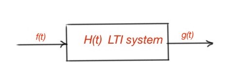Figure 1. Representation of periodic function going through the LTI system.

Here, ${\int }_{–\infty }^{\infty }h\left(\phi \right)f\left(\phi \right)d\phi$ and $\sum _{–\infty }^{\infty }h\left[\phi \right]f\left[\phi \right]$ are system functions of the LTI system.

When we are considering signals, it is important to consider exponential functions of the type $e^{–jw}$ and their frequency response of the LTI system. For a continuous-time system ${\int }_{–\infty }^{\infty }h\left(t\right)e^{–jwt}dt$ , for a discrete-time system $\sum _{–\infty }^{\infty }h\left[\phi \right]e^{–jwn}$ are the frequency responses. Moving to the signals with Fourier representation, for the Fourier coefficients the output function will be $c_{n}H\left(jwn\right)$.[1]

More educational tutorials can be accessed via Reddit community r/ElectronicsEasy.

[1] “Signals and systems”, 2nd edition, 1997. Alan V. Oppenheim, Allan S. Willsky.