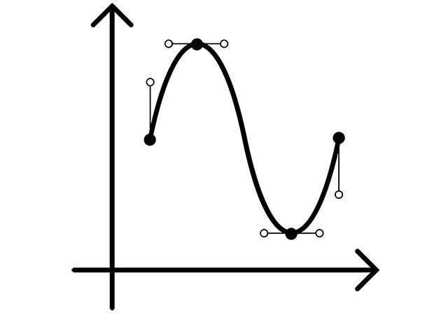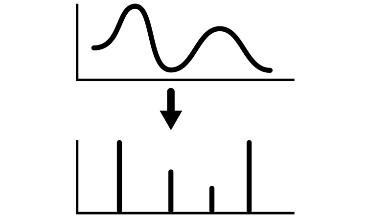
Fourier transform for discrete-time periodic function

Here we consider Fourier transform for discrete-time periodic function. Let’s consider the discrete-time Fourier-representation of a function $f [n] = \frac{1}{N} \sum_{- \infty}^{\infty} a_{n} e^{j n \frac{2 π}{n} K}$ , where $a_{n} = \frac{1}{N} \sum_{- \infty}^{\infty} F (j w) e^{- j n \frac{2 π}{N} k}$ and $F (j w) = {\sum x [n] e^{- j n \frac{2 π}{N} k}}_{- \infty}^{\infty}$ .

The pair of equations that are called the Fourier pair for discrete-time functions $x [n] = \frac{1}{2 π} \int_{- \infty}^{\infty} F (j w) e^{j w n}$ and $F (j w) = \sum_{k = - \infty}^{\infty} x [n] e^{- j n \frac{2 π}{N} k}$ .

The Fourier transform for discrete-time periodic function has properties that are similar to the properties of a continuous-time Fourier transformation listed below.

Linearity. For the two pairs of Fourier transformation $f_{1} [n] = \frac{1}{2 π} \int_{- \infty}^{\infty} F_{1} (j w) e^{j w n} d w$ and $f_{1} (j w) = \sum_{k = - \infty}^{\infty} f [n] e^{- \frac{j n 2 π}{N} k}$ , $f_{2} [n] = \frac{1}{2 π} \int_{- \infty}^{\infty} F_{2} (j w) e^{j w n}$ and $F_{2} (j w) = \sum_{k = - \infty}^{\infty} f_{2} [n] e^{- \frac{j n 2 π}{N} k}$ for the function $a f_{1} [n] + b f_{2} [n]$ the Fourier transformation will be $a F_{1} (j w) + b F_{2} (j w)$ .
Periodicity. For the pair of Fourier transformations $f [n] = \frac{1}{2 π} \int_{- \infty}^{\infty} F (j w) e^{j w n} d w$ and $F (j w) = {\sum f}_{- \infty}^{\infty} [n] e^{- \frac{j n 2 πk}{N}}$ . The Fourier transformation of two functions are different within a period are identical $F (j w) = F (j (w + 2 π))$ .
Shifting property. If we have a shifted discrete-time function $f_{1} [n - n_{0}]$ so the corresponding Fourier transformation for this function will be $e^{- j w n_{0}} F_{1} (j w)$ .
Conjugation. For the pair $f [n]$ and $F (j w)$ there is a conjugation rule that for the function $f^{*} [n]$ the Fourier transformation is: $F (- j w)$ .
Differencing property. Let’s consider the discrete-time function $f [n]$ , so for the sum $\underset{n}{\sum f [n]}$ will correspond the Fourier transformation $\frac{1}{1 - e^{- j w}} F (j w) + πF (j 0) \sum_{k = - \infty}^{\infty} δ (w - 2 πk)$ .
Time reverse. Let’s consider a function $f [n]$ and it’s Fourier transformation $F (j w)$ , so for the function $f [- n]$ the Fourier transformation will be $F (- j w)$ .
Expansion property. For the discrete-time function f[an] the function of the Fourier transformation will be $F (j w a)$ .
Differentiation property. If we have a discrete-time function $f [n]$ , that is characterised with the Fourier transformation $F (j w)$ , so the differential of the Fourier transformation $\frac{d F (j w)}{d w}$ will correspond to the function $\frac{n f [n]}{j}$ .
Parseval formula. For the discrete-time function $f [n]$ with Fourier transformation $F (j w)$ the following Parseval relation is valid ${\sum {|f [n]|}^{2}}_{- \infty}^{\infty} = \frac{1}{2 π} \int_{2 π} {|F (j w)|}^{2}$ . This means that the signal energy can also be integrated by frequency. As for the continuous-time signals ${|F (j w)|}^{2}$ is the energy density spectrum.
Convolution property. Let’s consider two discrete-time functions $f [n]$ and $h [n]$ with Fourier transformations $F (j w)$ and $H (j w)$ , and discrete-time function $g [n] = f [n] * h [n]$ that is the convolution of two discrete-time functions. So the function g[n] will have the Fourier transformation $G (j w) = F (j w) H (j w)$ .
Multiplication property. Let’s consider two discrete-time functions $f_{1} [n]$ and $f_{2} [n]$ with the multiplication product $h [n]$ . Let’s assume they are characterised with Fourier transformations $F_{1} (j w)$ and $F_{2} (j w)$ . So the Fourier transformation of the function is $h [n]$ is $H (j w) = \frac{1}{2 π} \int_{2 π} F_{1} (j φ) F_{2} (j (φ - w)) d φ$ .

Let’s consider the LTI system, which is characterised with the equation $\underset{k}{\sum b_{k} g [k] = \underset{k}{\sum a_{k} f [k]}}$ . Functions $h [k]$ and $f [k]$ are characterised with the Fourier transformations $F (j w)$ and $G (j w)$ $G (j w)$ . So, the LTI system is characterised by the Fourier transformation: $H (j w) = \frac{F (j w)}{G (j w)}$ .[1]