Thévenin equivalent circuit and maximum power transfer

After the introduction of the SMU ADALM1000 let’s continue with the third part of our ADALM1000 series with some small, basic measurements.

By Doug Mercer and Antoniu Miclaus, Analog Devices

Now let’s get started with the next experiment.

Objective

The objective of this lab activity is to verify Thévenin’s theorem by obtaining the Thévenin equivalent voltage (VTH) and Thévenin equivalent resistance (RTH) for the given circuit, and then to verify the maximum power transfer theorem.

Background

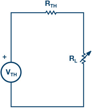
Thévenin’s theorem is a process by which a complex circuit is reduced to an equivalent circuit consisting of a single voltage source (VTH) in series with a single resistance (RTH) and a load resistance (RL). After creating the Thévenin equivalent circuit, the load voltage VL or the load current IL may be easily determined.

One of the principal uses of Thévenin’s theorem is to replace a large portion of a circuit, often a more complicated and uninteresting part, with a simple equivalent. The new simpler circuit enables rapid calculations of the voltage, current, and power than the more complicated original circuit is able to deliver to a load. The theorem also helps to choose the optimal value of the load (resistance) for maximum power transfer.

Figure 2. Thévenin equivalent circuit of Figure 1.

The maximum power transfer theorem states that an independent voltage source in series with a resistance, $R_{S}$ , or an independent current source in parallel with a resistance RS delivers a maximum power to the load resistance, $R_{L}$ , when $R_{L} = R_{S}$ .

In terms of a Thévenin equivalent circuit, maximum power is delivered to the load resistance $R_{L}$ when $R_{L}$ is equal to the Thévenin equivalent resistance, $R_{T H}$ , of the circuit.

Materials

ADALM1000 hardware module
Various resistors (100 Ω, 330 Ω, 470 Ω, 1 kΩ, and 1.5 kΩ)

Procedure

1. Verifying Thévenin’s theorem:

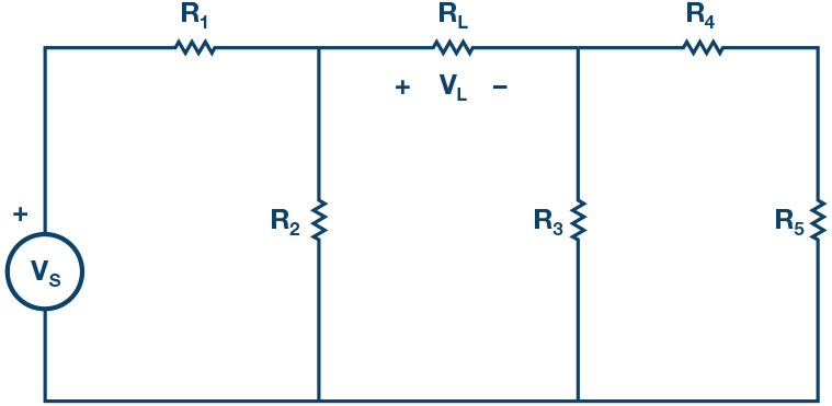
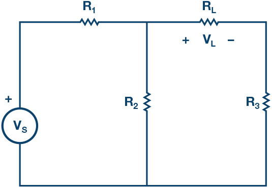
a) Construct the circuit of Figure 2 using the following component values:

$R_{1} = 330 Ω$
$R_{2} = 470 Ω$
$R_{3} = 470 Ω$
$R_{4} = 330 Ω$
$R_{5} = 1 k Ω$
$R_{L} = 1.5 k Ω$
$V_{S} = 5 V$

b) Accurately measure the voltage $V_{L}$ across the load resistance using the ALM1000 voltmeter tool. Use the voltmeter tool by connecting channel CA to the positive node of $V_{L}$ and connect channel CB to the negative $V_{L}$ will be the difference between CA volts and CB volts. This value will later be compared to the one you will find using the Thévenin equivalent.

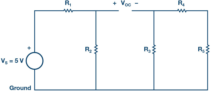
c) Find $V_{T H}$ : Remove the load resistance, $R_{L}$ , and measure the open circuit voltage, $V_{O C}$ , across the Use the voltmeter tool by connecting channel CA to the positive node of $V_{O C}$ and connect channel CB to the negative node. $V_{O C}$ will be the difference between CA volts and CB volts. This is equal to $V_{T H}$ . See Figure 4.

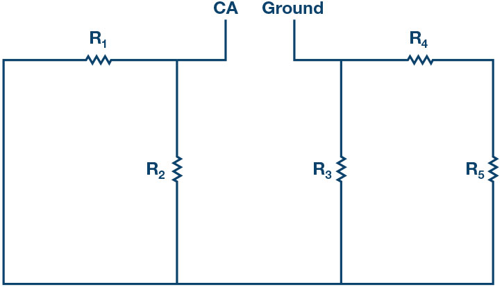
Figure 4. Measuring the Thévenin voltage.

d) Find $R_{T H}$ : Remove the source voltage $V_{S}$ and construct the circuit as shown in Figure Use the ALM1000 ohmmeter tool to measure the resistance looking into the opening where $R_{L}$ was. This gives $R_{T H}$ . Make sure there is no power applied to the circuit before measuring with the ohmmeter and that the ground connection has been moved as shown.

Figure 5. Measuring the Thévenin resistance, RTH.

e) Obtaining $V_{T H}$ and $R_{T H}$ , construct the circuit of Figure 2. Create the value of $R_{T H}$ using a series and or parallel combination of resistors from your parts Using the meter-source tool, connect channel CA for the $V_{T H}$ source and set the value to what you measured for $V_{T H}$ in Step c.

Figure 6. Thévenin equivalent construction.

f) With $R_{L}$ set to the $5 k Ω$ used in Step b, measure the $V_{L}$ for the equivalent circuit and compare it to the $V_{L}$ obtained in Step b. This verifies the Thévenin theorem.

g) Optional: repeat Step 1b to Step 1f for $R_{L} = 2.2 k Ω$ .

2. Verifying the maximum power transfer theorem:

a) Construct the circuit as in Figure 7 using the following values:

$V_{S} = 5 V$
$R_{1} = R_{2} = 470 Ω$
$R_{3} = 1 k Ω$
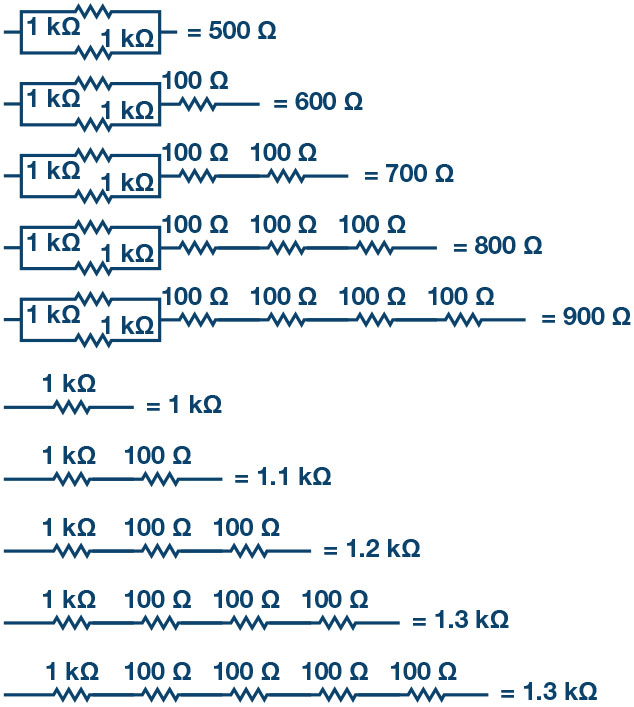
$R_{L} =$ combinations of $1 k Ω$ and $100 Ω$ resistors (Figure 8)

Figure 7. Circuit for maximum power theorem.

b) Use the voltmeter tool by connecting channel CA to the positive node of $V_{L}$ and connect channel CB to the negative node across $R_{L}$ . $V_{L}$ will be the difference between CA volts and CB

c) To find the value of $R_{L}$ for which maximum power is transferred, vary the load resistances by constructing series/parallel combinations of $1 k Ω$ and $100 Ω$ for $R_{L}$ between $R_{L}$ to $1400 Ω$ in $100 Ω$ steps, as shown in Figure 8. For each value of $R_{L}$ , write down $V_{L}$ .

d) Calculate the power for each load resistor value using $P_{L} = \frac{{V_{L}}^{2}}{R_{L}}$ . Then, interpolate between your measurements to calculate the load resistor value corresponding to the maximum power ( $P_{L}$ -max). This value should be equal to $R_{T H}$ of circuit in Figure 7 with respect to load terminals.

Questions

Using voltage division for the circuit of Figure 2, calculate $V_{L}$ . Compare it to the measured Explain any differences.
Calculate the maximum power transmitted to the load $R_{L}$ obtained for the circuit of Figure 3.

You can find the answers at the StudentZone blog.

Notes

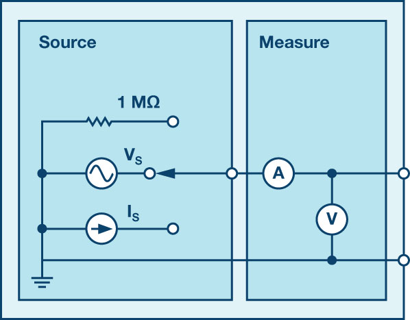
As in all the ALM labs, we use the following terminology when referring to the connections to the ALM1000 connector and configuring the hardware. The green shaded rectangles indicate connections to the ADALM1000 analog I/O connector. The analog I/O channel pins are referred to as CA and CB. When configured to force voltage/measure current, –V is added (as in CA-V) or when configured to force current/measure voltage, –I is added (as in CA-I). When a channel is configured in the high impedance mode to only measure voltage, –H is added (as in CA-H).

Scope traces are similarly referred to by channel and voltage/current, such as CA-V and CB-V, for the voltage waveforms, and CA-I and CB-I for the current waveforms.

We are using the ALICE rev 1.1 software for those examples here.

File: alice-desktop-1.1-setup.zip. Please download here.

The ALICE desktop software provides the following functions:

A 2-channel oscilloscope for time domain display and analysis of voltage and current
The 2-channel arbitrary waveform generator (AWG) controls.
The X and Y display for plotting captured voltage and current voltage and current data, as well as voltage waveform histograms.
The 2-channel spectrum analyzer for frequency domain display and analysis of voltage
The Bode plotter and network analyzer with built-in sweep generator.
An impedance analyzer for analyzing complex RLC networks and as an RLC meter and vector
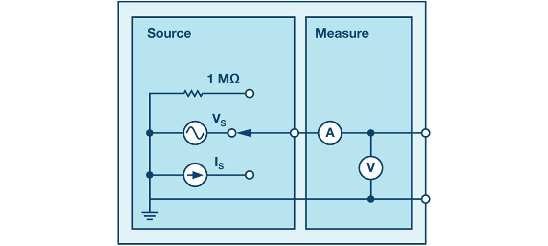
A dc ohmmeter measures unknown resistance with respect to known external resistor or known internal 50 Ω.
Board self-calibration using the AD584 precision 2.5 V reference from the ADALP2000 analog parts kit.
ALICE M1K voltmeter.
ALICE M1K meter source.
ALICE M1K desktop tool.

For more information, please look here.

Note: You need to have the ADALM1000 connected to your PC to use the software.

Antoniu Miclaus [antoniu.miclaus@analog.com] is a system applications engineer at Analog Devices, where he works on ADI academic programs, as well as embedded software for Circuits from the Lab® and QA process management. He started working at Analog Devices in February 2017 in Cluj-Napoca, Romania. He is currently an M.Sc. student in the software engineering master’s program at Babes-Bolyai University and he has a B.Eng. in electronics and telecommunications from Technical University of Cluj-Napoca.

Doug Mercer [doug.mercer@analog.com] received his B.S.E.E. degree from Rensselaer Polytechnic Institute (RPI) in 1977. Since joining Analog Devices in 1977, he has contributed directly or indirectly to more than 30 data converter products and he holds 13 patents. He was appointed to the position of ADI Fellow in 1995. In 2009, he transitioned from full-time work and has continued consulting at ADI as a Fellow Emeritus contributing to the Active Learning Program. In 2016 he was named Engineer in Residence within the ECSE department at RPI.