Parallel LC resonance

Objective: The objective of this activity is to examine the oscillations of a parallel LC resonant circuit. In addition, the self-resonance of a real inductor will be examined.

By Doug Mercer and Antoniu Miclaus, Analog Devices

Background: A resonant circuit, also called a tuned circuit, consists of an inductor and a capacitor together with a voltage or current source. It is one of the most important circuits used in electronics. For example, a resonant circuit, in one of many forms, allows us to tune into a desired radio or television station from the vast number of signals that are around us at any time.

A network is in resonance when the voltage and current at the network input terminals are in phase and the input impedance of the network is purely resistive.

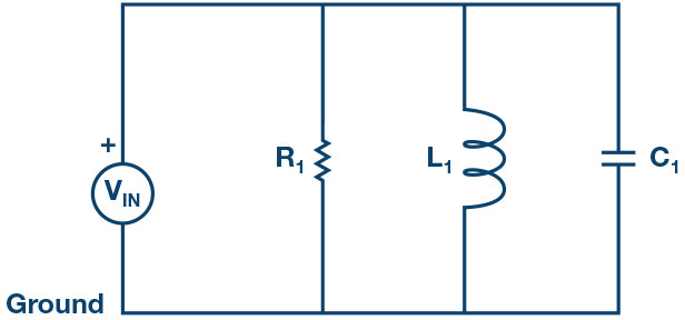
Consider the parallel RLC circuit of Figure 2. The steady-state admittance offered by the circuit is $Y = \frac{1}{R} + j (w C - \frac{1}{w C})$ .

Resonance occurs when the voltage and current at the input terminals are in phase. This corresponds to a purely real admittance, so that the necessary condition is given by $w C - \frac{L}{w} = 0$ .

The resonant condition may be achieved by adjusting L, C, or ω. Keeping L and C constant, the resonant frequency ωo is given by $w_{0} = \frac{1}{\sqrt{L C}} \frac{r a d}{s}$ .

Or $f_{0} = \frac{1}{2 π \sqrt{LC}} H z$ .

Materials

ADALM1000 hardware module
Solderless breadboard and jumper wires
One 4.7 mH inductor (or larger)
One 10 μF capacitor
One 1 kΩ resistor
One small signal diode (1N914)

Directions

First, a quick diversion to examine using a diode as a switch.

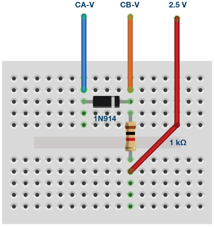
Set up the circuit shown in Figure 3 on your solderless breadboard. Configure the AWG CH-A to output a sine wave with a frequency 100 Hz and Min value of 0.5 V and a Max value of 4.5 V (V p-p = 4 V). Set up the horizontal time scale to view two full cycles of the sine wave on Channel A and so that the signal looks as large as possible without going off the screen. Configure Channel B in Hi-Z Mode and connect it to where R1 connects to D1.

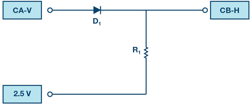
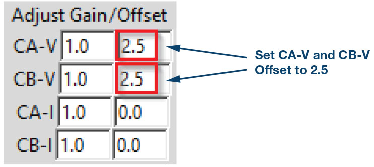
Figure 4. Diode test circuit breadboard connections.

Hand draw the circuit diagram, carefully labeling the connections from the ALM1000 for CH-A, 2.5 V, and CH-B, and include it in your lab report. From the Curves drop-down menu, select the CA-V, CA-I, and CB-V traces for display. On the right-hand side of the scope screen, enter 2.5 for the CA-V and CB-V offset adjustment. This is because in this experiment we are referencing all the measurements to the 2.5 V common rail. Also enter 0 for the CH-A and CH-B vertical position settings (along the bottom of scope screen). The vertical scale should now be centered on 0 and go from –2.5 to +2.5.

Click Run. You will not be given this direction at every step. It is assumed that you will know you have to start and stop the sweeps at various steps in the experiments.

Use the Math drop-down menu and add a trace that displays the difference between CH-A and CH-B. For this experiment, make sure the vertical scales are the same for all three signals being displayed.

Observe what happens to the sine wave as it passes through the diode and the current being supplied by Channel A. Describe the waveforms in a sentence. Save the display and copy and paste it into your lab report. Label the input voltage (produced by the AWG source), the input current supplied by the source, and the output voltage (across the resistor). Also show the magnitude of each signal at key points (do not assume that the reader can easily figure it out from the scales on the plot).

1. Based on this observation, what is the function of a diode?

Switch the AWG A shape to square wave output and make sure the oscilloscope shows a few cycles of the signal. Save this waveform and include it in your report. Again, fully annotate your plot.

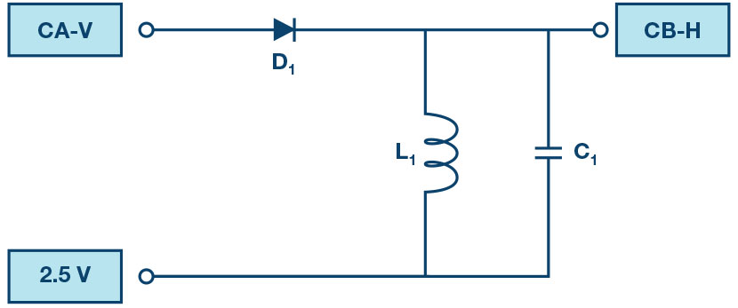
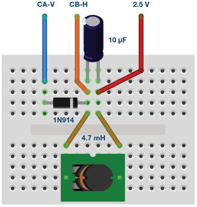
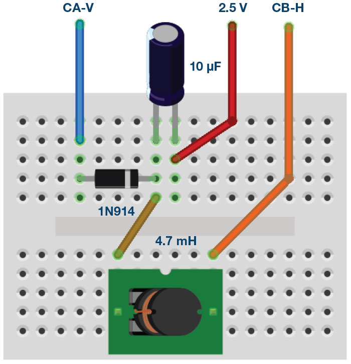
Reconfigure the breadboard circuit with the diode, inductor, and capacitor, as shown in Figure 5. Mentioned earlier, connect Channel A to the diode and Channel B across the capacitor and inductor.

Figure 6. LC resonator test circuit breadboard connections

2. Calculate the frequency at which the circuit should oscillate.

Now you will use the oscilloscope to measure the frequency at which the circuit actually oscillates. When you apply the 100 Hz square wave, the LC circuit will oscillate immediately after the falling edge of the square wave. Change the horizontal position or hold-off time to place the oscillations at the left of the grid (so you can see as much of the oscillation as possible).

Change your Horizontal Time/Div in order to easily observe and measure the period of oscillation. With the sweeping stopped (red stop button), left clicking on the display grid will add marker points to the display. The delta in voltage and time between the last two markers will also be displayed. Use the delta time between adjacent peaks or valleys of the oscillations to get the period. Save the display and include it in your report (fully annotated).

3. From the period, determine the frequency at which the circuit oscillates.

The frequency should be approximately equal to the calculated frequency. If not, check the component values in your circuit and calculations. Note in your report if the frequency you measured is a little smaller or a little larger than the one given by the formula.

Do you see why the diode was used? A diode passes current in one direction only. During the half of the square wave above the 2.5 V rail, the diode conducts and energizes the LC resonator. For the half of the square wave below the 2.5 V rail, the diode does not conduct, so the LC resonator is effectively isolated from the AWG source and is free to oscillate.

4. Does the waveform have a constant amplitude, or does it grow or decay?

Describe the waveform in words and discuss why it differs from simple theory. Look up the specification sheet for the inductor and see if you can find the characteristic that causes the growth or decay (here is where reading the entire write-up will help you).

Now adjust the square wave so that its Min value is 0.5 V and Max value is

3.5 V (V p-p = 3 V).

Repeat the measurements you just made, again saving and annotating the data plots. Explore other combinations of Min and Max values for the square wave.

5. What is different about the voltages measured? Compare to the previous plot.

Energy Storage

The voltage across the parallel capacitor/inductor should be a decaying sinusoid (also called a damped sine wave). A realistic model of an inductor includes a series resistance. Some of the energy in the resonator is converted to heat when current flows through this resistance. This loss of energy results in the amplitude of the osculation decaying over time.

In addition to the resonator voltage, we would also like to measure the capacitor and inductor currents. First, to obtain the current in the capacitor, we can make use of the following formula $I_{C} = C \frac{d v}{d T}$ .

To calculate the discrete time derivative of the capacitor voltage, we can subtract two consecutive time samples and divide by the change in time between samples. The time between samples is simply 1/sample rate. For the ALM1000, the sample rate is 100 kSPS or 10 μsec per sample. The value of C1 is 10 μF, which just happens to cancel when divided by the 10 μsec. The formula gives the current in amps. To plot in mA, simply multiply by 1000. Set the Math axis to I-A and enter the following for the Math formula $(V_{B U F F} B [t] - V_{B U F F} B [t - 1]) x 1000$ .

Looking at the schematic in Figure 5, again we note that when the diode is off and the resonator is oscillating, the only place for the current in the capacitor to go is in the inductor. So $I_{L} = I_{C}$ .

From the inductor current waveform and the capacitor voltage waveform, we can calculate the instantaneous energy in each component. Using the Math formula feature, plot the two energy waveforms as a function of time.

The first will be the energy in the inductor. The units for inductance is joules per ampere square. So the energy in joules is $E_{L} = \frac{1}{2} L I^{2}$ .

One half of the 4.7 mH inductor value is 0.00235 H. A 4.7 mH inductor with 40 mA flowing through it is storing 0.00000376 joules of energy or 3.76 μJ (microjoules). A very small number so we will scale it by 106. To plot the energy in the inductor (in microjoules), enter the following for the Math formula $E_{L} = 2350 x {(V_{B U F F} B [t] - V_{B U F F} B [t - 1])}^{2}$ .

The second will be the energy in the capacitor. The units for capacitance is coulombs squared per joule. The number of coulombs stored on the capacitor is equal to the capacitance times the voltage. So the energy in joules is $E_{C} = \frac{1}{2} C V^{2}$ .

One half of the 10 μF inductor value is 0.000005 F. A 10 μF capacitor charged to 1 V has 0.000005 joules of energy or 5 μJ (microjoules). A very small number so we will scale it by 106. To plot the energy in the capacitor (in microjoules), enter the following for the Math formula 5x ${(V_{B U F F} B [t])}^{2}$ .

Save and fully annotate these plots in your report.

Discuss the two energy values, how they change with time, and their relation to one another. For example, when is the energy contained mostly or entirely in the inductor? When is it contained mostly or entirely in the capacitor? What trends over time from cycle to cycle do you see? Be as quantitative as you can, but mostly address the overall picture.

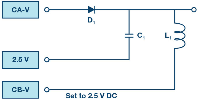
The current in the inductor can be directly measured by disconnecting the inductor from the fixed 2.5 V power rail and connecting it to the output of AWG Channel B as shown in Figure 7. Set AWG CH-B to SVMI Mode and Shape dc with the Max value set to 2.5 V. Select the CB-I trace from the Curves menu.

Compare the trace you get with the calculated capacitor current (and by the same inference we just made, the inductor current). Note any differences and explain why.

How could you use this measurement technique to directly measure the current in the capacitor?

Figure 7. Directly measuring the inductor current.

Appendix:

Figure 8. Directly measuring the inductor current breadboard connections.

Self-Resonance

All real inductors possess a built-in capacitance, called a parasitic capacitance. The inductor acts as if it has a capacitance connected in parallel with it. This is sometimes called the winding capacitance.

Remove the capacitor from your breadboard and measure the frequency at which the inductor oscillates. Adjust the horizontal time scale as needed to clearly see the oscillation. You probably want to turn on Waveform Smoothing (under the options menu) when measuring the high frequency that the inductor self resonates at.

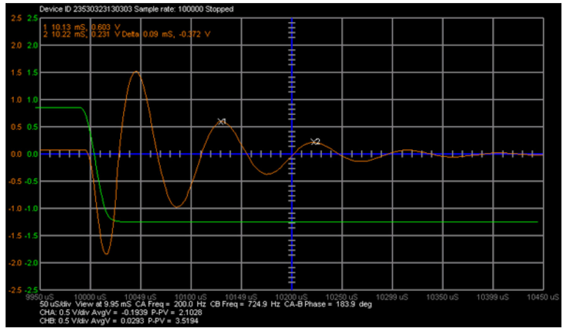
Self-Resonance Example

Figure 8 is a representative example of self-resonance waveform for a 4.7 mH inductor.

Questions

Calculate the value of the parasitic capacitance.
Inductors also have an internal series resistance that should not be ignored when they are modeled. What aspect of the oscillating signal you measured for the LC circuit is caused by the resistance?

Figure 10. Screen capture of step 5 with Time/Div set to 0.5 msec.

You can find the answers at the StudentZone blog.

Notes

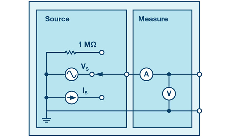
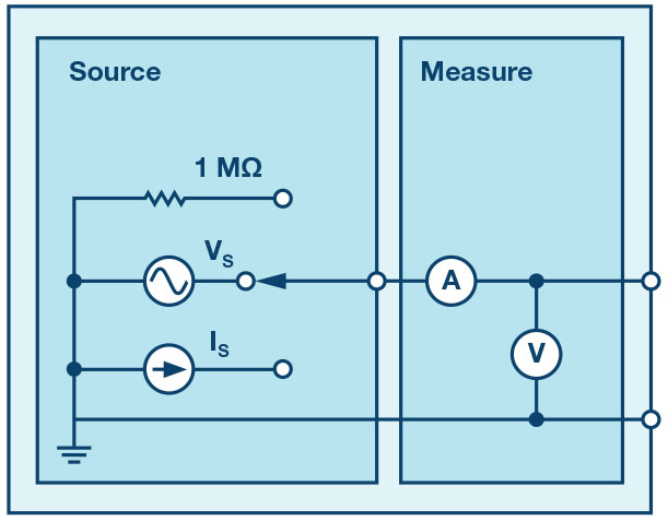
As in all the ALM labs, we use the following terminology when referring to the connections to the ALM1000 connector and configuring the hardware. The green shaded rectangles indicate connections to the ADALM1000 analog I/O connector. The analog I/O channel pins are referred to as CA and CB. When configured to force voltage/measure current, –V is added (as in CA-V) or when configured to force current/measure voltage, –I is added (as in CA-I). When a channel is configured in the high impedance mode to only measure voltage, –H is added (as in CA-H).

Scope traces are similarly referred to by channel and voltage/current, such as CA-V and CB-V for the voltage waveforms, and CA-I and CB-I for the current waveforms.

We are using the ALICE Rev 1.1 software for those examples here. File: alice-desktop-1.1-setup.zip. Please download here.

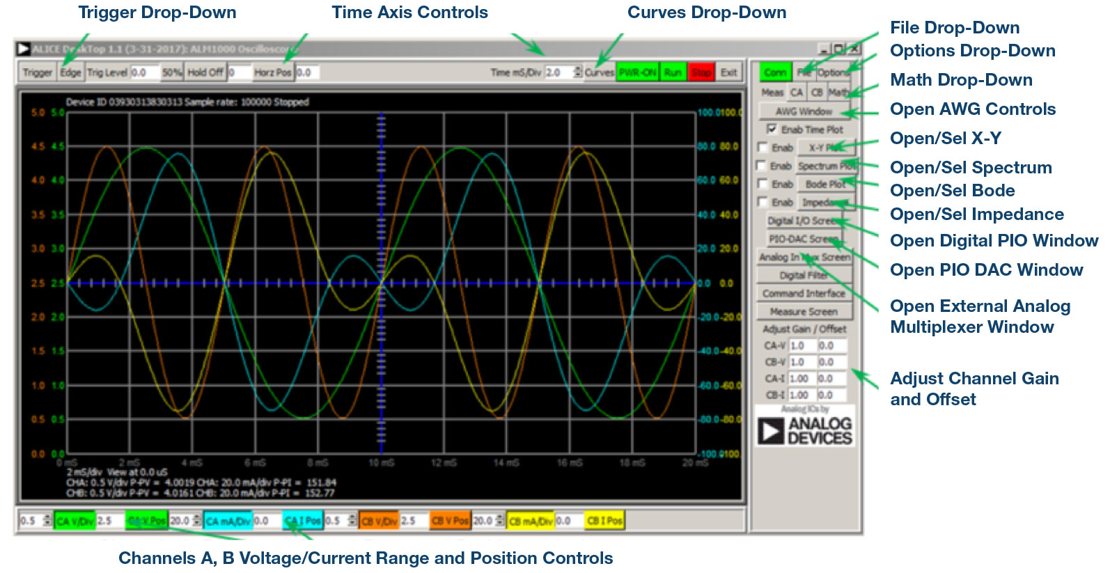
The ALICE Desktop software provides the following functions:

A 2-channel oscilloscope for time domain display and analysis of voltage and current waveforms.
The 2-channel arbitrary waveform generator (AWG) controls.
The X and Y display for plotting captured voltage and current vs. voltage and current data, as well as voltage waveform histograms.
The 2-channel spectrum analyzer for frequency domain display and analysis of voltage waveforms.
The Bode plotter and network analyzer with built-in sweep generator.
An impedance analyzer for analyzing complex RLC networks and as an RLC meter and vector voltmeter.
A dc ohmmeter measures unknown resistance with respect to known external resistor or known internal 50 Ω.
Board self-calibration using the AD584 precision 2.5 V reference from the ADALP2000 analog parts kit.
ALICE M1K voltmeter.
ALICE M1K meter source.
ALICE M1K desktop tool.

For more information, please look here.

Note: You need to have the ADALM1000 connected to your PC to use the software.

Doug Mercer [doug.mercer@analog.com] received his B.S.E.E. degree from Rensselaer Polytechnic Institute (RPI) in 1977. Since joining Analog Devices in 1977, he has contributed directly or indirectly to more than 30 data converter products, and he holds 13 patents. He was appointed to the position of ADI Fellow in 1995. In 2009, he transitioned from full-time work and has continued consulting at ADI as a Fellow Emeritus contributing to the Active Learning Program. In 2016 he was named Engineer in Residence within the ECSE department at RPI.

Antoniu Miclaus [antoniu.miclaus@analog.com] is a system applications engineer at Analog Devices, where he works on ADI academic programs, as well as embedded software for Circuits from the Lab® and QA process management. He started working at Analog Devices in February 2017 in Cluj-Napoca, Romania.

He is currently an M.Sc. student in the software engineering master’s program at Babes-Bolyai University and he has a B.Eng. in electronics and telecommunications from Technical University of Cluj-Napoca.