The transmission line as parallel planes, stripes and microstripes

 Parallel planes or stripes is the most general example of transmission line. Schematically it is depicted below. The parallel stripes can carry TEM, TM and TE waves.

For analysis of TEM waves we must resolve the Laplace equation ${\nabla }^2\Phi (x,y)=0$. Let’s consider the case where the bottom stripe is grounded and the top stripe carries potential $V_0$. Geometry of the transmission lines allows us to assume that the solution will be as a linear equation for the potential $\Phi (x,y)=Ay+B$. Applying the boundary conditions $Ф(x,y)=\frac{V_{0y}}{d}$. So the electric field is $E(x,y)=-\frac{V_{0y}}{d} e^{–j\omega \sqrt{\mathrm{\mu \epsilon }z}}{\mathit{e}}_{\mathbf{y}}$ where e_y is the radius-vector. The magnetic field is $H(x,y)=\frac{V_{0x}}{d}\sqrt{\frac{\epsilon }{\mu } }{e}^{–\mathrm{jw}\sqrt{\mathrm{\mu \epsilon }z}}{\mathit{e}}_{\mathbf{x}}$, where e_x is a radius-vector. The potential difference between two stripes or the voltage is $V={{\int }_0}^d E_y\mathrm{dy}=V_0{e}^{–\mathrm{jw}\sqrt{\mathrm{\mu \epsilon }}}$, the induced current is $I={{\int }_0}^W H_x\mathrm{dx}=\frac{W}{d}\sqrt{\frac{\epsilon }{\mu }}{V}_0 e^{–j\omega \sqrt{\mathrm{\mu \epsilon }}}$, the characteristic impedance is: $Z_0=\frac{V}{I}=\frac{d}{W}\sqrt{\frac{\mu }{\epsilon }}$.

The same as we discussed before, TE waves are characterised as $E_Z=0, H_Z\ne 0$. Applying the reduced wave equation we can find the $E_x$ and $H_Z$. And the TE waves will have the following characteristics:

Cut-off wave number $$\begin{gathered} k_{\mathrm{nm}}=\omega \sqrt{\mathrm{\mu \epsilon }} \\ {k}_{\mathrm{cnm}}=\frac{\mathrm{n\pi }}{d} \end{gathered}$$ .
Propagation constant ${\beta }_{\mathrm{nm}}=\sqrt{k^2–\frac{{\mathrm{n\pi }}^2}{d^2}}$ .
Cut-off wavelength $$\begin{gathered} {\lambda }_{\mathrm{cnm}}=\frac{2\pi }{k_{\mathrm{cnm}}} \\ {\lambda }_{\mathrm{gnm}}=\frac{2\pi }{\beta } \end{gathered}$$.
Phase velocity   $v_{\mathrm{pnm}}=\frac{\omega }{\beta }$ .
Dielectric attenuation constant ${\alpha }_{dnm}=\frac{k^2\tan \sigma }{2\beta }$.
$$\begin{gathered} E_{\mathrm{znm}}=0 \\ {H}_{\mathrm{znm}}=\mathrm{Bcosn}\frac{\mathrm{\pi ny}}{d}{e}^{–\mathrm{j\beta z}} \\ {E}_{\mathrm{xnm}}=-\frac{\mathrm{j\omega \mu }}{k_c}\mathrm{Bsin}\frac{\mathrm{\pi ny}}{d}{e}^{–\mathrm{j\beta z}} \\ {E}_{\mathrm{ynm}}=\; 0 \\ {H_x}_{\mathrm{nm}}=\; 0 \\ {H}_{\mathrm{ynm}}=\; –\frac{\mathrm{j\beta }}{k_c}\mathrm{Bsin}\frac{\mathrm{\pi n}}{d}{e}^{–\mathrm{j\beta z}} \end{gathered}$$ Impedance  $Z_{\mathrm{TEnm}}=\frac{k}{\beta }\sqrt{\frac{\mu }{\epsilon }}$ .

The power flow for TE waves is $P_{\mathrm{TE}}=\frac{\mathrm{Re}}{2}{{\int }_0}^W{{\int }_0}^d E_x{H}_y*\mathrm{dxdy}$, the attenuation constant is $\alpha =\frac{2{k_c}^2{R}_s}{\mathrm{k\beta d}}\sqrt{\frac{\epsilon }{\mu }}$.

TM waves are characterised by $H_z=0,E_z\ne 0$. Resolving wave equation $(\frac{{\partial }^2}{{\partial }^{2}y}+{k_c}^2) E_z(x,y)=0$, we can obtain $E_z(x,y)$ and the remaining TM wave characteristics apply the boundary conditions.

Cut-off wave number   $$\begin{gathered} k_{\mathrm{nm}}=\omega \sqrt{\mathrm{\mu \epsilon }} \\ {k}_{\mathrm{cnm}}=\frac{\mathrm{n\pi }}{d} \end{gathered}$$ .
Propagation constant   ${\beta }_{\mathrm{nm}}=\sqrt{k^2–\frac{{\mathrm{n\pi }}^2}{d^2 }}$ .
Cut-off wavelength  $$\begin{gathered} {\lambda }_{\mathrm{cnm}}=\frac{2\pi }{k_{\mathrm{cnm}}} \\ {\lambda }_{\mathrm{gnm}}=\frac{2\pi }{\beta } \end{gathered}$$ .
Phase velocity  $v_{\mathrm{pnm}}=\frac{\omega }{\beta }$ .
Dielectric attenuation constant ${\alpha }_{dnm}=\frac{k^2\tan \sigma }{2\beta }$.
$$\begin{gathered} E_{\mathrm{znm}}=A\sin \frac{\mathrm{\pi ny}}{d}{e}^{–\mathrm{j\beta z}} \\ {H}_{\mathrm{znm}}=\; 0 \\ {E}_{\mathrm{xnm}}=0 \\ {E}_{\mathrm{ynm}}=\; –\frac{\mathrm{j\beta }}{k_c}\mathrm{Acos}\frac{\mathrm{\pi ny}}{d}{e}^{–\mathrm{j\beta z}} \\ {H}_{\mathrm{xnm}}=\frac{\mathrm{jw\epsilon }}{k_c}\mathrm{Acos}\frac{\mathrm{\pi ny}}{d}{e}^{–\mathrm{j\beta z}} \\ {H}_{\mathrm{ynm}}=\; 0 \end{gathered}$$ Impedance $Z_{\mathrm{TMnm}}=\frac{\beta }{k}\sqrt{\frac{\mu }{\epsilon }}$.

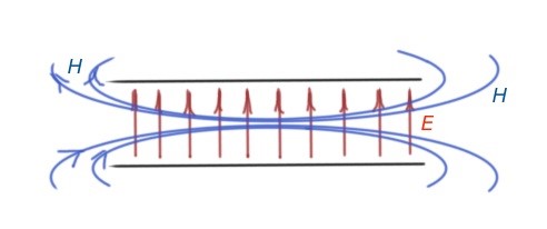
The power flow in the transmission line can be obtained via $P_{\mathrm{TE}}=-\frac{\mathrm{Re}}{2}{{\int }_0}^W{{\int }_0}^d E_y{H}_x*\mathrm{dxd}y$, the power dissipated in the transmission line is $P_d=R_s{{\int }_0}^W {J_S}^2\mathrm{dx}$. And the attenuation constant is $\alpha =\frac{2{\mathrm{kR}}_s}{\mathrm{\beta d}}\sqrt{\frac{\mu }{\epsilon }}$. Figure 2 shows the field lines for TEM waves, the $T{E}_n$ and $T{M}_n$ wave field line can be calculated for certain values on n.

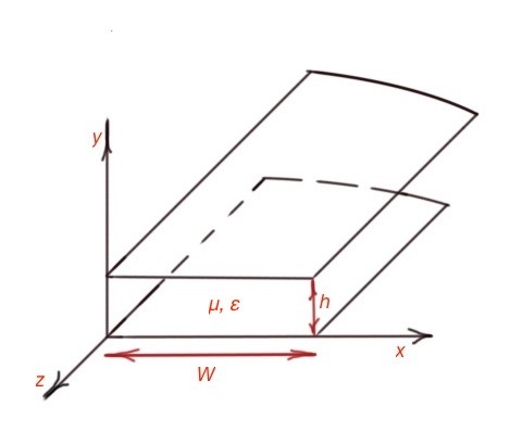
The related geometry transmission line is a stripline which can be seen in Figure 3, where the dielectric material fill the space between two conducting plates. A stripline is usually manufactured with several techniques including etching and photolithographic fabrication. The basic operation mode of a stripline is TEM waves mode.

Striplines the same as other transmission line geometries support all modes orders, but in practice they are always limited for some practical application by the voltage applied to the plates, or by the distance between them. It is not easy to apply the Laplace equation and wave equation techniques to resolve the characteristics of a stripline. Striplines can be calculated numerically. Striplines are characterised by the following formulas:

$v_p=\frac{c}{\sqrt{{\epsilon }_r}}, \mathrm{\beta =}\frac{w}{v_p}, Z_0=\frac{\sqrt{{\epsilon }_r}}{\mathrm{cC}}$, where c is the velocity of light in a free-space. Usually the characteristic impedance for a stripline has a more complex form and fully depends on the geometry of the stripline $Z_0=\frac{30\pi }{\sqrt{{\epsilon }_r}} \frac{h}{W_e+0.441h}$.

The parameter W_e is the effective width, and it can be calculated in the following way $\frac{W_e}{h}=\frac{W}{h}–\left\{\begin{array}{l}0, \frac{W}{h}>0.35\\ (0.35–\frac{W}{h}), \frac{W}{h}<0.35\end{array}\right.$

A variety of catalogues and reference books give the $\frac{W}{h}$ characteristics for a stripline. And these characteristics allow us to calculate the stripline width when designing the stripline. $\frac{W}{h}=\frac{30\pi }{\sqrt{{\epsilon }_r}{Z}_0}-0.441$ when $\sqrt{{\epsilon }_r}{Z}_0<120Ohm$ and $\frac{W}{h}=0.85-\sqrt{1.441}–\frac{30\pi }{\sqrt{{\epsilon }_r}{Z}_0}$ when $\sqrt{{\epsilon }_r}{Z}_0>120\mathrm{Ohm}$.

Attenuation constant of the practical stripline also depends on the stripline geometry $\alpha =\frac{2{.7*10}^{-3}{R}_s{\epsilon }_r{Z}_0}{30\pi (h–d)} (1+\frac{2W}{h–d}+\frac{1}{\pi }\frac{h+d}{h–d} \ln \frac{2h–d}{d})$, when $\sqrt{{\epsilon }_r{Z}_0}<120Ohm$ and $\alpha =\frac{0.16R_s}{Z_{0}h} (1+\frac{h}{0.5W+0.7a} (0.5+\frac{0.414a}{W}+\frac{1}{2\pi } \ln \frac{4\mathrm{\pi W}}{a}$. The formulas above can be used for practical usage when designing a stripline.

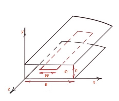
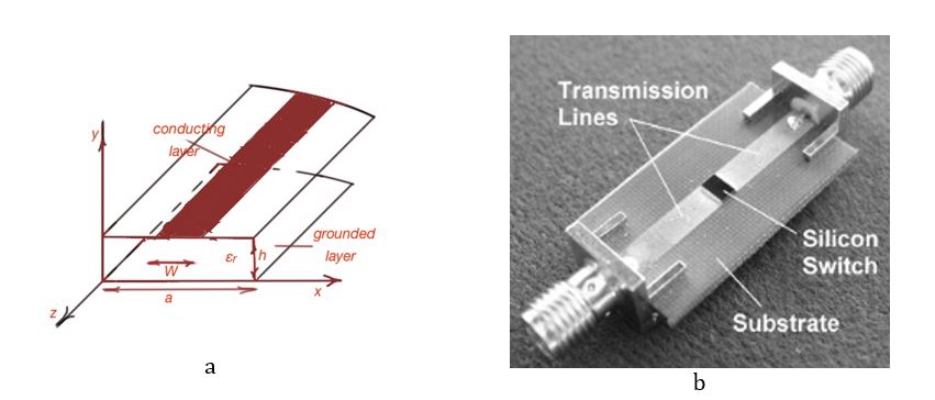
The microstrip is the most popular transmission line in RF and microwave, depicted in Figure 4. It is fabricated with standard printed circuit techniques, can be miniaturised and integrated into any system, and is less expensive in production.

The microstrip consists of the conducting plate and dielectric layer. The outer conductor is a single flat metal ground-plane. The inner conductor is a metal plane separated from the outer plane by the dielectric layer.

The practical microstrip has a very thin dielectric layer and the resulting electromagnetic fields are quasi-TEM. So all the solutions for TEM waves are not exactly static, but quasi-static and can be described with an approximation. A microstrip line is characterised with an effective dielectric constant, that can be seen in all the approximation formulas for TEM waves for microstrips. The effective dielectric constant depends on the microstrip geometry and dielectric constant of the dielectric layer, and it is always less than the dielectric constant of the layer: ${\epsilon }_{\mathrm{ef}}=\frac{{\epsilon }_r+1}{2}+\frac{{\epsilon }_r-1}{2}\frac{1}{\sqrt{1+12\frac{h}{W}}}$.

The characteristic impedance for the microstrip will depend on the microstrip geometry $Z_0=\frac{60}{\sqrt{{\epsilon }_{\mathrm{ef}}}}\ln \frac{24h^2+W^2}{4\mathrm{hW}}, \mathrm{if} \frac{W}{h}\le 1, \mathrm{and} Z_0=\frac{120\pi }{\sqrt{{\epsilon }_{\mathrm{ef}}}(\frac{W}{h}+1.393+0.677 \ln (\frac{W}{h}+1.444))}, \mathrm{where} \frac{W}{h}\ge 1$.

The reverse procedure of obtaining the ratio $\frac{W}{h}$ from Z₀ is possible as well. Attenuation of the microstrip is ${\alpha }_d=\frac{k_0{\epsilon }_r({\epsilon }_{\mathrm{ef}}-1)\tan \sigma }{2\sqrt{{\epsilon }_{\mathrm{ef}}}({\epsilon }_r-1)}$  (the dielectric losses of the transmission line), and ${\alpha }_c=\frac{\sqrt{{\displaystyle \frac{w{\mu }_0}{2\sigma }}}}{Z_{0}W}$ (the conduction losses of the transmission lines).

(«Microwave engineering», David M.Pozar, 4th edition, Wiley; “The ARRL Handbook for radio communications 2015”, ARRL; www.researchgate.net, the optically activated switch in the transmission line.)