This post covers properties of LTI system. Linear-time invariant systems, that were partially discussed before, play an important role in describing signals. Generally speaking, any process can be described with the idea of Linear-Time Invariant systems. So here we will consider LTI system properties in detail.
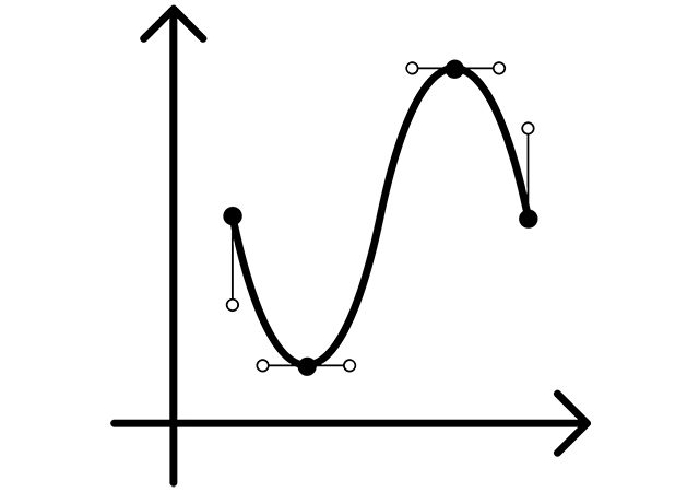
Let’s consider continuous-time function . We can divide it into fractions as depicted in Figure 1. Each fraction can be described with function .
Let’s assume that , then . Let’s assume that is the response of LTI system to the input function. So the LTI system output for the function will be .
This expression is called a convolution integral for a system. Convolution is the mathematical operation of obtaining the third function from two others, describing how one of the function changes the form of another. Convolution can also be written as .
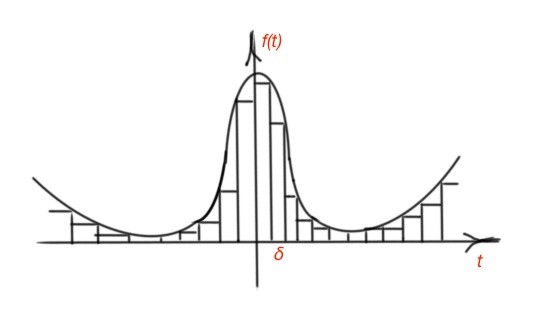
Figure 1.Continuous-time function represented with the impulses.
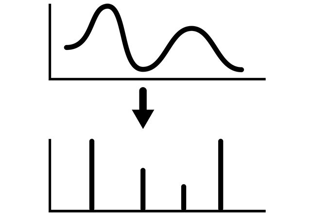
Let’s represent discrete-time signal as the row of unit impulses, as depicted in Figure 2. Mathematically it will be . As we know, function is the function equal to zero everywhere except zero. In our case, we can consider shifted function with weight in every considered point. So here the considered function is a superposition of functions with corresponding weights.
Let’s assume that the LTI system response for function is , then the output function of the LTI system will be . This expression is called a convolution sum for a system. Convolution is the mathematical operation of obtaining the third function from two others, describing how one of the function changes the form of another. Convolution can also be written as .
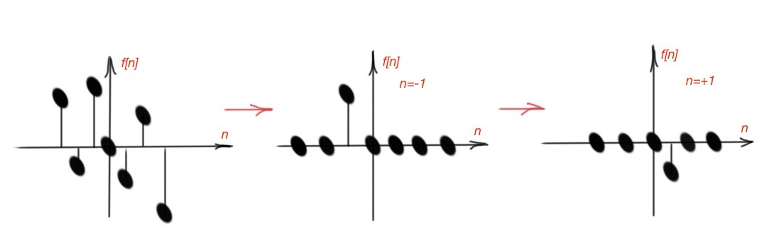 Figure 2. The discrete-time function represented with impulses.
Here are some properties of linear-time invariant systems convolution.
- Commutative property. For the input functions and , and LTI system responses and the following expressions are valid: and .
- Distributive property. For the input functions and , and LTI system responses , and , the following expressions are valid: and .
- Associative property. For the input functions and , and LTI system responses , and , the following expressions are valid:, and .
- Inversion property. If the LTI system is an inverting function, then and , here are responses of the input and output functions in the case of continuous-time and discrete-time functions.
- Stability property. Let’s assume that the input function is limited, so , then considering the convolution sum and integral we can understand if the output function is stable. , so the output function will be stable if the integral . Similarly we can show for the discrete-time function is stable if the sum . [1]
More educational tutorials can be accessed via Reddit community r/ElectronicsEasy.
[1] “Signals and systems”, 2nd edition, 1997. Alan V. Oppenheim, Allan S. Willsky.