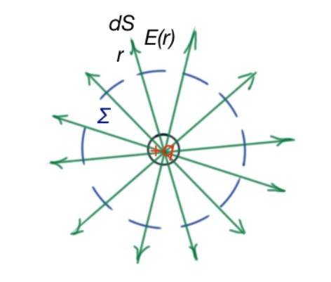
The Coulomb Law and superposition principle can lead to divergence theorem which is valid for bilateral, axial and spherical charged objects. Let’s divide the surface , by the parts . Module of is equal to the square of (Figure below), and is directed along the normal .
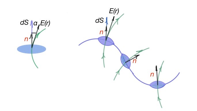
Elementary flow dФ of the electric field through the piece of surface is a .
En is a projection on the normal to the surface element . To simplify this case, the electric field flow is a scalar multiplication of the vectors and :
So the electric field that flows through the surface
Electric field flow has the following properties:
- Electric field flow through the surface is proportional to the number of electric field lines through this surface. As flow is a vector term and vector direction has to be taken into account.
- Superposition principle is valid for electric field flow, and states that if surface is the amount of charges then total electric field flow is an algebraic sum of electric field flow , created by every single dot charge of the surface (Figure below).
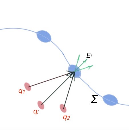
Based on the conclusions above, Gauss theorem can be introduced. Gauss theorem states the following: electric field flow in a vacuum through the closed surface ∑ is proportional to the total charge of this surface:
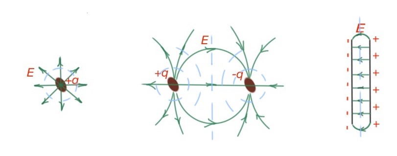
Let’s consider several cases of charged surfaces.
- Spherical surface surrounds point charge. (Figure below). Electric field structure for this case is radial, and it is reverse proportional to the square of distance from point charge to some point in space. In this case, for every small piece of spherical surface vector coincides to the Then we can switch from the sign of sum to the integral.
2. Let’s consider a single charge shifted from the centre of the sphere (Figure below). In this case angles between vectors and for every point on the sphere are different, and electric field has different values. Electric field flow through the sphere is equal to the quantity of electric field lines, crossing its surface. This means that the result should be the same as for case 1. We can also use integration to find the electric field flow through the surface. According to the Gauss theorem
. Here is a measure of solid angle for . So .3. System of N point charges is placed inside and outside of the closed random form surface. Every single charge inside the surface creates electric field flow .
Every single charge outside the surface does not create an electric field. So for N charges inside the surface .
In the case of extended one-, two- or three-dimensional charge, integration must be used in Gauss theorem instead of sum sign. So curved, surface or volume integral will be used:
where –are linear, surface and volume charge density; – space areas have distributed charge.
The most comfortable way to use Gauss theorem is when the system is characterised with flat, axis or spherical symmetry – where you can switch from the surface integral to the multiplication of scalar quantities and .
Task 3: Prove that the electric field outside the uniformly charged sphere (dielectric , ) on the distance bigger than R, sphere radius, is the same as the electric field of a single point charge q.
Task 4: Determine electric field of the uniformly charged infinite cylinder with permittivity , and radius : a. inside the cylinder; b. outside the cylinder. is a charge volume density, r is a distance from the cylinder axis.
There is a potential difference in electric field id scalar value. It is also an electric field characteristic, and it is very useful, as it is easier to use scalar quantities. We consider all the charges in an electrostatic field, when electric forces in electrostatic fields are conservative. Forces are considered to be conservative if their work does not depend on the object of the force movement trajectory. This work is determined only by initial and final coordinates of a moving object.
Stationary point electric charge is the source of central field force. According to the superposition principle, work wasted on the movement of a single charge in the system of stationary charges is equal to the algebraic sum of works from all the separate charges. This field is also a field of conservative forces. So work of electrostatic forces characterises the electric field, and depends on the considered charge.
The potential difference between two points in electric field 1 and 2 is the ration of work (of electric field) needed to move considered charge q from point 1 in point 2, to the value of considered charge .
The measurement unit is Volts (V). So work needs to be done to move charge q from point 1 to point 2:
A potential difference is the energy characteristics of an electric field.
Let’s consider the point in space where the electric field is absent and .
So, the electric field energy needed to move the charge from point to a random point of the electric field is .
Let’s express the field work as characteristics of the field E. and
Let’s consider a potential of point charge. First, assuming . The point in space we are calculating the electric field potential is distanced from the charge to the distance r. To simplify the task, let’s assume the electric field lines are in a radial straight line from the charge. Then .
In this case . Potential energy of a point charge in the electric field is .
For two point charges and interaction energy is .
Equipotential surfaces are energy characteristics of an electric field that characterises the moving charge in an electric field. Work along these surfaces is 0. It’s at its maximum along the directions, where there is maximum density of equipotential surfaces. Electric fields here is also maximum. Equipotential surfaces and electric field lines are perpendicular. (Figure below). Work of any charge movement along the equipotential surface is 0, so it’s possible only if the electric field is directed normally to the surfaces. There is a very easy mathematical explanation
then . Here are equipotential surfaces for cases we discussed above. (Figure below).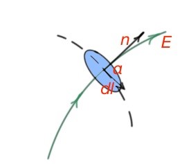
Potential of system point charges
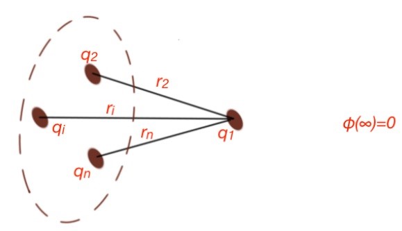
Field potential of a system of point charges is characterised by the superposition principle .
The proof of this statement is based on the facts that the potential of a field is work that needs to move a charge to the point of space where the field is equal to 0. And in the fact that work is an additive term. For system of charges in the field (Figure below).
Let’s use the potential superposition principle for calculating field potential on the axis of a charged circle, with radius R and charge q, where x is the distance from the circle’s centre. (Figure below).
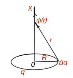
The circle can be divided to the point charges . And according to the superposition principle .