There are two methods of magnetic induction B calculation. The first method is using the Biot-Savart-Laplace and induction superposition principle. The second method is using the B vector circulation theorem, which will be explained below.
It is very easy to use this theorem with cylindrical, sphere or flat symmetry of a conductor. Vector circulation by the enclosed loop A is
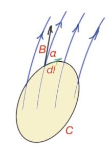
Figure 28. (B,dr) is a projection of B on the vector dr, which is integral algebraic sum of the projections of B on the dr vector, when the loop A is a set of fragments. It is important to note that we cannot derive the loop to the electrons, because an electron is an accelerating particle. However, magnetic field devices in our approximation are characterised by a velocity component. Thus, vector B circulation theorem states the following:
Magnetic field B circulation by the enclosed loop A, is proportional to the algebraic sum of currents going through this loop
If there is a distributed current flowing through the surface Ω surrounded by the closed loop or path A, then
should be replaced by
where j is a density of a current flow through the surface Ω enclosed by the loop A.
If we generalise the circulation statements for simple cases, it will lead us to the most complex case.
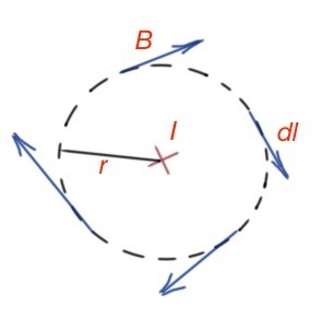
- Considering a wire with electric current, we choose the path A perpendicular to the conductor – this path will correlate to the one of magnetic induction lines. Figure 29. Then
By the Biot-Savart-Laplace Law B(r) this conductor is then This result corresponds to the theorem we stated before.
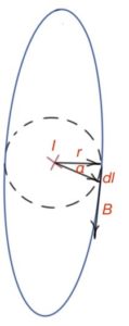
2. 2. Let’s consider the case with the same straight wire, but taking a closed path with a random form. Then
The magnetic induction for the wire is
then
3. Let’s consider the case when the conductor is outside of the path A. Figure 31. The path with be divided into two parts, then the result will be evident:
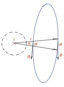
4. If the path A is oriented with some angle to the conductor and has a random form, we can also divide projections of B on the dr – to parallel and perpendicular components:
(perpendicular component – result related to previous case).
5. In the case of several conductors crossing the loop, we can generalise the result above and make an algebraic sum of the magnetic induction circulation integrals. This generalisation will lead us to the result
Let’s resolve some examples using the theorem of magnetic field circulation.
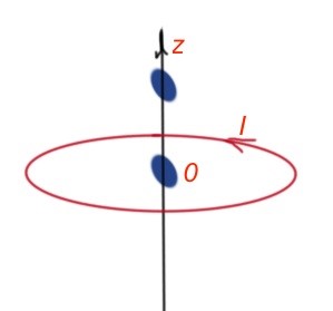
For radius-vector r coordinates are (0,0,z), for radius vector r1 coordinates are (Rcosα,Rsinα,0). Then for dr1 (-Rsinαdα,Rcosαdα,0) and r- r1=(-Rcosα,-Rsinα,z). For r-r1 × dr1 we have (zcosα,zsinα,R)Rdα.
For
then
Magnetic fields outside of the solenoid are very small, and nearly all the magnetic fields ars concentrated inside of it. The magnetic field of the solenoid is uniform.
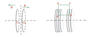
Sometimes wires form complex structures. So how do we use the Biot-Savart-Laplace Law in this case? To resolve these cases the structure can be divided into segments. And Biot-Savart-Laplace Law can be applied individually to each segment. Then for a complex structure we get:
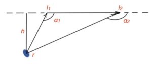
Let’s consider the segment of a wire depicted on the Figure c. rdr=dhdl, where h is the line from the point where we are estimating the magnetic field to the wire segment, or its extrapolation. l is coinciding with the wire segment. As h is perpendicular to the wire segment, then hxl=h*l. And drxr=dhxdl. Then
Here
So
Let’s express l1 and l2 with known variables – h and α.
Then
For the given straight segment of wire
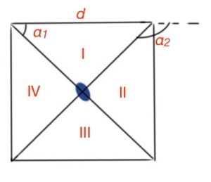
The square sides are d, the
Magnetic field at the centre of the square
(magnetic field for the triangle).