Classification of signals

Classification of signals

Classification of signals: Even and odd signals

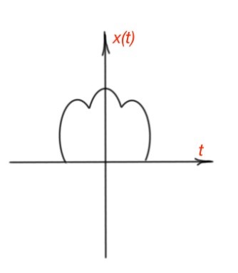
This post covers topic of classification of signals.The continuous-time and discrete-time electromagnetic signals are called even if they are identical to their counterparts on the time scale, i.e.  $x\left(t\right)=x(–t)$ and $x\left[n\right]=x[–n]$. The continuous-time and discrete-time signals are called odd if they are opposite to their counterparts on the time scale, i.e. $x\left(t\right)=–x\left(t\right)$ and $x\left[n\right]=–x\left[n\right]$. The feature of odd signals is that zero is equal when $t=0$ and $n=0$. The odd and even signals are depicted below for continuous-time signals. 

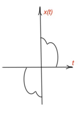
Any signal can be broken into even and odd parts: $\mathrm{Ev}\left\{x\right(t)\}=\frac{1}{2}\left[x\right(t)+x(-t)]$ and $\mathrm{Od}\left\{x\right(t)\}=\frac{1}{2}\left[x\right(t)-x(-t)].$.

Classification of signals: Exponential and sinusoidal electromagnetic signals

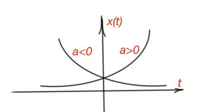
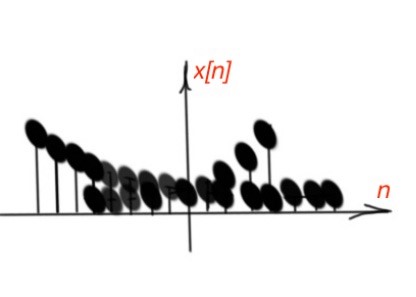
The continuous-time exponential signals are $x(t)={\mathrm{Ce}}^{\mathrm{at}}$ where $C$ and a are complex numbers. If $C$ and a are real complex numbers then the function $x\left(t\right)$ is real and there are two behaviours of the function: if a is positive $x\left(t\right)$ is an increasing exponential function, if the a is negative, then $x\left(t\right)$ is a decreasing exponential function. (Figure 3).

If a is an imaginary complex number, then the function $x(t)=e^{\mathrm{j\omega t}}$. This function is periodic, and it means that $e^{\mathrm{j\omega t}}=e^{\mathrm{j\omega }(t+T)}$. It does mean that $e^{\mathrm{j\omega T}}=1$. That may happen if $\omega =0$ or T is a fundamental period $T=\frac{2\pi }{\omega }$.

The signals $e^{\mathrm{j\omega t}}$ and $e^{–\mathrm{j\omega t}}$ have the same fundamental period. The exponential function also can be written in the form $e^{\mathrm{j\omega t}}=\mathrm{cos\omega t}+\mathrm{jsin\omega t}$. As exponential function is periodic, then $e^{\mathrm{j\omega t}}=1$, then $\mathrm{\omega T}=2\mathrm{\pi k}$ where k is an integer, and $\omega =\frac{2\mathrm{\pi k}}{T}$ where k is an integer. We can also include a new term of harmonically related functions $f(t)=e^{\mathrm{jk\omega t}}$, where k is an integer with fundamental frequency $\omega =\frac{2\mathrm{\pi k}}{T}$.

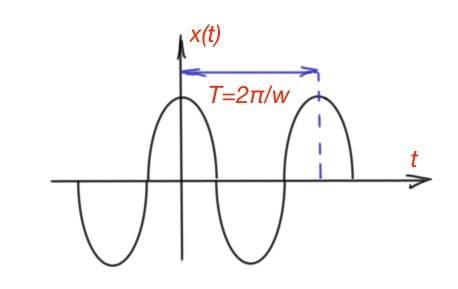
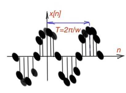
The other type of electromagnetic signal is a sinusoidal signal $x\left(t\right)=A\cos (\omega t+\phi )$. The angular frequency here is $\omega =2\pi f$, where $f$ is a frequency, and $\phi$ is a phase shift. Sinusoidal signals are also periodic functions with a fundamental period $T$. A sinusoidal signal can be written in the following form: $\mathrm{Acos}(\mathrm{\omega t}+\phi )=\frac{A}{2}{e}^{\phi }{e}^{\mathrm{j\omega t}}+\frac{A}{2}{e}^{–\phi }{e}^{–\mathrm{j\omega t}}$. And also from the stated above $\mathrm{Acos}(\mathrm{\omega t}+\phi )=\mathrm{ARe}\{e^{(\mathrm{j\omega t}+\phi )}\},\mathrm{Asin}(\mathrm{\omega t}+\phi )=\mathrm{AIm}\{e^{(\mathrm{j\omega t}+\phi )} \}$ (Figure 4).

The total energy of a periodic exponential function over the period T is $E{{=\int }_0}^T(e^{\mathrm{j\omega t}}{)}^2\mathrm{dt}=T$. As there is an infinity quantity of the periods in the sin/cos function, so the total energy of exponential or sinusoidal function is infinite. The average power is $P=\frac{1}{TE}=1$. The average power of the exponential or sinusoidal function is still equal to 1, no matter how many periods there are.

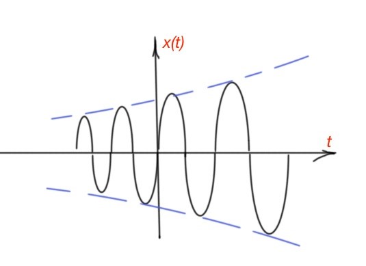
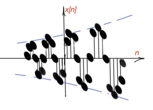
Let’s consider the most general complex exponential function $x(t)={\mathrm{Ce}}^{\mathrm{at}}$ where $C$ is a complex number and a is a complex number. So that $C=|C|e^{\mathrm{j\theta }}$, and $a=r+\mathrm{j\omega }.\mathrm{C=|}{C}_1|e^{j(\mathrm{\omega t}+\theta )}=|C_1|\cos (\mathrm{\omega t}+\theta )+j|C_1\left|\sin \right(\mathrm{\omega t}+\theta ),\mathrm{where}|C_1|=|C|e^{\mathrm{rt}}$. So there are three cases: $r=0$, the function $x\left(t\right)$ is pure sinusoidal. For $r>0$ the sinusoidal is inscribed in the increasing exponential function (Figure 5). For $r<0$ the sinusoidal is inscribed in the decreasing exponential function.

Discrete-time signals can also be complex sinusoidal and exponential. Discrete-time complex exponential signals are $x[n]={\mathrm{Ce}}^{\mathrm{\alpha n}}$, C is a complex number, α can be complex or an integer. When $C$ and $\alpha$ are real, the function decreases or increases exponentially, depending on the sign of $\alpha$.

The sign of the function magnitude varies depending on the sign of C. (Figure 6). If the α=jω is an imaginary number, then $x[n]={\mathrm{Ce}}^{\mathrm{j\omega n}}$ This function can be written as $e^{\mathrm{j\omega n}}=\mathrm{cos\omega n}+\mathrm{jsin\omega n}, \mathrm{in} \mathrm{the} \mathrm{mean}\mathrm{time} \cos (\mathrm{\omega n}+\phi )=\frac{1}{2}{e}^{\mathrm{j\phi }}{e}^{\mathrm{j\omega n}}+\frac{1}{2}{e}^{–\mathrm{j\phi }}{e}^{–\mathrm{j\omega n}}$.

As with continuous-time functions, discrete-time periodic functions are characterised with infinite energy and finite average power. The discrete-time periodic function can be written as $x[n]={\mathrm{Ce}}^{\mathrm{j\theta }}(\cos (\mathrm{\omega n}+\phi )+\mathrm{jsin}(\mathrm{\omega n}+\phi \left)\right)$, where Figure 7 depicts different cases of this function behaviour.

The discrete-time complex exponential function is a periodic function, with period 2π, so $e^{j(\mathrm{\omega n}+2\pi )}=e^{\mathrm{j\omega n}}{e}^{j2\pi }=e^{\mathrm{j\omega n}}$ And here is a big difference between discrete-time and continuous-time functions regarding periodicity. The continuous-time function will have distinct values for different values of frequency $\omega +2\pi , \omega +4\pi$ and so on. The discrete-time functions have the same values for different values of frequency $\omega +2\pi , \omega +4\pi$ and so on.

As far as discrete-time complex exponential function is periodic, then the following should be true: $e^{\mathrm{j\omega n}}=e^{\mathrm{j\omega }(n+N)}, \mathrm{so} e^{\mathrm{j\omega N}}=1,\mathrm{then} \mathrm{\omega N}=2\mathrm{\pi m}$, where m is an integer. So the fundamental period for discrete-time function is $N=\frac{2\pi }{\omega }m$. This statement also does not have the same meaning for continuous-time functions. Both functions should have an undefined fundamental period for fundamental frequency $\omega =0$. For discrete-time functions we can also define harmonically-related functions as $x[n]={e^{\mathrm{jk}}}^{\left(\frac{2\pi }{\omega }\right)}n$, for different $k=0,1,2,...$

Classification of signals: Unit-step and unit-impulse functions

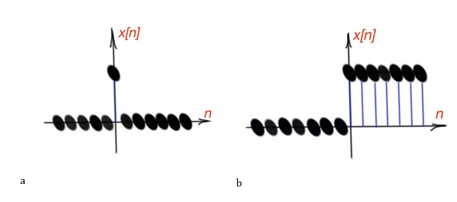
Another important type of signals are unit-step and unit-impulse signals. These signals can be continuous-time and discrete time functions. The discrete-time impulse function is $\delta [n]=\left\{\begin{array}{l}0,n\ne 0\\ 1,n=0\end{array}\right.$. The discrete-time step function is $x\left[n\right]=\left\{\begin{array}{l}0,n<0\\ 1,n\ge 0\end{array}\right.$.

These functions are shown in Figure 9. There is a direct relationship between discrete-time unit step and pulse functions – the discrete-time unit impulse is the first difference of discrete-time unit step, $\delta \left[n\right]=x\left[n\right]–x\left[n–1\right]$. The unit step function is the running sum of the unit impulse function $x\left[n{{]=\sum }_{m=-\infty }}^n\delta \right[n]$.

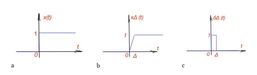
The unit impulse and unit step functions are related to the following: $x\left[n\right]\delta \left[n\right]=x\left[n\right]\delta \left[0\right]$. Continuous-time functions can also be unit pulsed and step. They are represented similarly as: $x\left(t\right)=\left\{\begin{array}{l}1,t>0\\ 0,t<0\end{array}\right.$, the unit-impulse continuous-time function is discontinuous at $t=0$.

They are related to each other: $x(t{{)=\int }_{-\infty }}^t \delta (t)\mathrm{dt}$ and reverse $\delta (t)=\frac{\mathrm{dx}\left(t\right)}{dt}$. But there is an important note – since the impulse function $\delta \left(t\right)$ is undefined at $t=0$, we must calculate the derivative for $\delta \left(t\right)$ at $t\to 0$. So it can be represented with the following way: ${\delta }_{∆} (t)=\underset{∆\to 0}{\lim } \frac{{\mathrm{dx}}_{∆}\left(t\right)}{∆t}$.

Graphically unit-step and impulse-step functions are presented in Figure 10. The impulse-unit continuous-time function is $\delta (t)=\underset{∆\to 0}{\lim }{\delta }_{∆}(t)$. The impulse-unit function can also be scaled ${{\int }_{-\infty }}^t \mathrm{k\delta }\left(t\right)\mathrm{dt}=\mathrm{ku}\left(t\right)$. Another interpretation of unit-step function with the time shift, if we represent $\sigma =t–\tau$, then $x(t{{)=\int }_0}^{\infty } \delta (t–\sigma \left)d\right(\sigma )$. Similarly to discrete-time function $x\left(t\right)\delta \left(t\right)=x\left(0\right)\delta \left(t\right)$.

Continuous-time and discrete-time electromagnetic systems

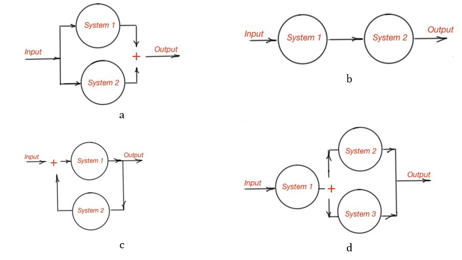
This system is a process where the input signal is transformed in some specific way by the system, resulting some specific output signal. Continuous-time system is a system where the continuous-time signal is applied and results in continuous-time output signals. The discrete-time system is a system that transforms discrete-time input signal into discrete-time output signal. Very often real systems are complex and are built as interconnections of simple subsystems. The types of interconnections are the series or cascade interconnection, the parallel interconnection, the series-parallel interconnection and feedback interconnection. All these interconnections are depicted graphically in Figure. 11.

System properties

This system is called memoryless when the output of the system for independent variables is dependent only on the input at the same moment of time. So, memoryless systems for continuous-time functions is $y(t)=x^2(t)+3x\left(t\right)$, or discrete-time function is $y\left[n\right]=8x\left[n\right]$.

The simplest memoryless system is an identical system when the output is identical to the input, $y\left(t\right)=x\left(t\right)$, or $y\left[n\right]=x\left[n\right]$. A discrete-time system with memory is a summer $y[n]=\sum _{k=-\infty }^n x[n]$, or it is also called an accumulator. Another example is delay, when $y\left[n\right]=x\left[n–1\right]$. The memory function of the system is the option of the input data storing at the moment that is different from current moment. Here is the memory concept on the summer : $y[n]=\sum _{k=-\infty }^{n-1} x[k]+x[n].$

A system is invertible if certain values of the input leads to certain values of the output. The invertible system is characterised with the inverse system. The inverse system is the system cascaded with the original system leading to a result equal to the input. For example, $y\left[n\right]=kx\left[n\right]$ is invertible system. The $y[n]=x^2 [n]$ is not an invertible system, as from here we can’t clearly know the sign of the original system.

The casual system is a system where the output values of the current time depends only on the value of the input at current time and previous time.

A system is called stable when the small inputs does not lead to output diversity.

A system is time invariant if the characteristics or behaviour of the system are fixed in time. The time shift of the input should provoke an identical time shift of the output.

A system is linear if the system input consists of the sum of the inputs, so the system output consists of the sum of outputs, where every output is the response of a particular input. Two features of the linear system is shown below. Let’s suppose that $y_1\left[n\right]$ is the output for the input $x_1\left[n\right]$ and the $y_2\left[n\right]$ is the output corresponding to the input $x_2\left[n\right]$. So the outputs:

1. For $x_1[n]+x_2[n]$ is the $y_1\left[n\right]+y_2\left[n\right]$ (additivity property);
2. For $a{x}_1$ is $a{y}_1$, where $a$ is any complex number (scaling property).

Here we can formulate the superposition property. If the set of discrete-system inputs $xk\left[n\right]$, for $k=1,2,3,...$ and the response of linear combination of these inputs are given by the sum $x[n]=\sum _k{a}_k x_k[n]$, where $a_k$ is an any complex number, then the superposition of outputs is $y[n]= \sum _k a_k{y}_k[n]$. The particular result of this feature is that if the input of the system is 0, then the output of the system will be 0 too.

More educational tutorials can be accessed via Reddit community r/ElectronicsEasy.

Discrete LTI systems