Rectangular waveguide

This post answers the question “What is rectangular waveguide?”. In order to find the transmission line impedance and the fields in the transmission line, we must resolve the Laplace equation of the potential, and take into account the Maxwell equation applied to the transmission line.

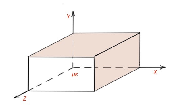
We studied the transmission line of the arbitrary form. Now we will take a look at the transmission lines having different geometry. Hollow rectangular transmission lines can perform only TE or TM waves. Let’s consider rectangular transmission lines (Figure 2). The transmission line is filled in with material with permeability and permittivity – see Figure 2.

For TE waves the $E_z=0$, and $H_Z\ne 0$. The $H_Z$ component can be found by resolving the Laplace equation. The formal type of z component of magnetic field $H_z(x,y)=({\mathrm{acosk}}_{x}x+{\mathrm{bsink}}_{x}x)({\mathrm{ccosk}}_{y}y+{\mathrm{dsink}}_{y}y)$. The constants can be calculated by taking into account the boundary conditions.

As well the electric and magnetic field components, cut-off frequency can be calculated using the magnetic field Hz using the formulas from the previous module. All the parameters of the TE mode are listed below. As we know when the operating frequency is larger than the cut-off frequency the TE waves are propagating, otherwise they are decaying exponentially.

The dominant TE mode occurs when m=1 and n=0. The TE mode does not exist when n=0 and m=0. The guide wavelength λg is the distance between the planes with the same phases, that define the phase velocity vp that defines the speed of the matter inside the transmission line.

For rectangular transmission lines the characteristics are chosen so the dominant TE wave propagates, so it’s reasonable to calculate characteristics of the only dominant wave of transmission line. As we know, the attenuation on the transmission line may only happen because of conduction or dielectric losses. The power loss for the transmission line can be found by integrating the surface current of the transmission line $P=\frac{R_S}{2}\int {J_S}^2 \mathrm{dl}$.

The attenuation constant $\alpha =\frac{P}{2P_{10}}$ is where P₁₀ is the power losses of the dominant mode. $k_{\mathrm{nm}}=\omega \sqrt{\mu \epsilon }$.

Cut-off wave number  $k_{\mathrm{cnm}}=\sqrt{(\frac{\mathrm{m\pi }}{a}{)}^2+(\frac{\mathrm{n\pi }}{b}{)}^2}$ .
Propagation constant  ${\beta }_{\mathrm{nm}}=\sqrt{k^2–{k_c}^2}$ .
Cut-off wavelength  $$\begin{gathered} {\lambda }_{\mathrm{cnm}}=\frac{2\pi }{k_c} \\ {\lambda }_{\mathrm{gnm}}=\frac{2\pi }{\beta } \end{gathered}$$ .
Phase velocity  $v_{\mathrm{pnm}}=\frac{\omega }{\beta }$ .
Dielectric attenuation constant :
$$\begin{gathered} {\alpha }_{\mathrm{dnm}}=\frac{k^2\mathrm{tan\delta }}{2\beta } \\ {E}_{\mathrm{znm}}=0 \\ {H_z}_{\mathrm{nm}}=\mathrm{Acos}\frac{\mathrm{m\pi x}}{a}\cos \frac{\mathrm{n\pi y}}{b}{e}^{–\mathrm{j\beta z}} \\ E_{\mathrm{xnm}}=\frac{\mathrm{j\omega \mu n\pi }}{{k_c}^{2}b}\mathrm{Acos}\frac{\mathrm{m\pi x}}{a}\sin \frac{\mathrm{n\pi y}}{b}{e}^{–\mathrm{j\beta z}} \\ {E}_{\mathrm{ynm}}= \frac{–\mathrm{j\omega \mu n\pi }}{{k_c}^{2}a}\mathrm{Acos}\frac{\mathrm{m\pi x}}{a}\sin \frac{\mathrm{n\pi y}}{b}{e}^{–\mathrm{j\beta z}} \\ {H}_{\mathrm{xnm}}=\frac{\mathrm{j\beta n\pi }}{{k_c}^{2}a}\mathrm{Acos}\frac{\mathrm{m\pi x}}{a}\sin \frac{\mathrm{n\pi y}}{b}{e}^{–\mathrm{j\beta z}} \\ {H}_{\mathrm{ynm}}= \frac{–\mathrm{j\beta n\pi }}{{k_c}^{2}b}\mathrm{Acos}\frac{\mathrm{m\pi x}}{a}\sin \frac{\mathrm{n\pi y}}{b}{e}^{–\mathrm{j\beta z}} \end{gathered}$$ Impedance  $Z_{\mathrm{TEnm}}=\frac{\mathrm{k\eta }}{\beta }$ .

TM mode is characterised by $H_Z=0$, $E_Z\ne 0$ and the $E_Z$ component can be found by resolving the Laplace equation. The formal type of z component of electric field $E_z(x,y)=({\mathrm{acosk}}_{x}x+{\mathrm{bsink}}_{x}x)({\mathrm{ccosk}}_{y}y+{\mathrm{dsink}}_{y}y)$. So field components and cut-off frequency can be calculated using the formulas from the previous section. The dominant TM wave is $T{M}_{11}$ that is characterised with the dominant frequency $f_{11}$. Attenuation constant in this case will be $\alpha =\frac{P}{2P_{11}}$. $k_{\mathrm{nm}}=\omega \sqrt{\mathrm{\mu \epsilon }}$.

Cut-off wave number $k_{\mathrm{cnm}}=\sqrt{(\frac{\mathrm{m\pi }}{a}{)}^2+(\frac{\mathrm{n\pi }}{b}{)}^{2 }}$ .
Propagation constant ${\beta }_{\mathrm{nm}}=\sqrt{k^2–{k_c}^2}$.
Cut-off wavelength $$\begin{gathered} {\lambda }_{\mathrm{cnm}}=\frac{2\pi }{k_c} \\ {\lambda }_{\mathrm{gnm}}=\frac{2\pi }{\beta } \end{gathered}$$ .
Phase velocity  $v_{\mathrm{pnm}}=\frac{\omega }{\beta }$.
Dielectric attenuation constant :
$$\begin{gathered} E_{\mathrm{znm}}=\mathrm{Bsin}\frac{\mathrm{m\pi x}}{a}\sin \frac{\mathrm{n\pi y}}{b}{e}^{–\mathrm{j\beta z}} \\ {H}_{\mathrm{znm}}=\; 0E_{\mathrm{xnm}}=\frac{–\mathrm{j\beta n\pi }}{{k_c}^{2}a}\mathrm{Bcos}\frac{\mathrm{m\pi x}}{a}\sin \frac{\mathrm{n\pi y}}{b}{e}^{–\mathrm{j\beta z}} \\ {E}_{\mathrm{ynm}}=\frac{\mathrm{j\beta n\pi }}{{k_c}^{2}b}\mathrm{Bsin}\frac{\mathrm{m\pi x}}{a}\cos \frac{\mathrm{n\pi y}}{b}{e}^{–\mathrm{j\beta z}} \\ {H}_{\mathrm{xnm}}=\frac{\mathrm{jn\omega \epsilon \pi }}{{k_c}^{2}b}\mathrm{Bsin}\frac{\mathrm{m\pi x}}{a}\cos \frac{\mathrm{n\pi y}}{b}{e}^{–\mathrm{j\beta z}} \\ {H}_{\mathrm{ynm}}=\frac{–\mathrm{jn\omega \epsilon \pi }}{{k_c}^{2}a}\mathrm{Bcos}\frac{\mathrm{m\pi x}}{a}\sin \frac{\mathrm{n\pi y}}{b}{e}^{–\mathrm{j\beta z}} \end{gathered}$$

Impedance $Z_{\mathrm{TMnm}}=\frac{\mathrm{\beta \eta }}{k}$.

Some manuals for RF and microwave devices contain extensive information about fields in the transmission lines and field lines and other waveguide characteristics.

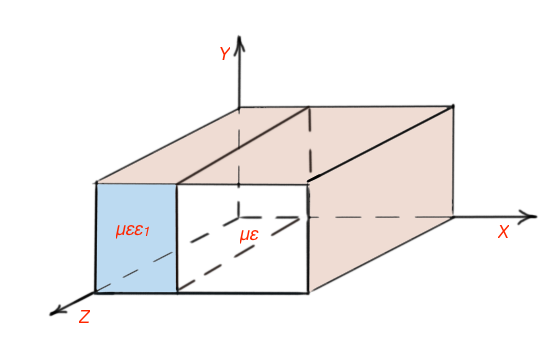
Some applications like impedance matching, demand partial filling of the waveguide with the dielectric (Figure 3). The boundary conditions will be different. $\left\{\begin{array}{l}\frac{{\partial }^2}{\partial x^2} +{k_d}^2 H_z=0, \mathrm{0\le }x\le a\\ \frac{{\partial }^2}{\partial x^2}+{k_a}^2 H_z=0, a\le x\le b \end{array}\right.$ , here $k_d$ and $k_a$ are the cut-off wave numbers for dielectric material and the non-dielectric part of a waveguide, and propagation constants $\beta =\sqrt{{{\mathrm{\epsilon k}}_0}^2–{k_d}^2}$ for dielectric and $\beta =\sqrt{{k_0}^2–{k_a}^2}$ for non-dielectric. Here $\left\{\begin{array}{l}{H}_z={\mathrm{Acosk}}_{d}x+{\mathrm{Bsink}}_{d}y,0\le x\le a\\ H_z={\mathrm{Ccosk}}_a(b–x)+{\mathrm{Dsink}}_a(b–y),a\le x\le b\end{array}\right.$.

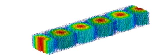
The Figure 4 shows simulation of electromagnetic fields in the rectangular waveguide.

More educational and technical posts you can read at our Reddit community r/ElectronicsEasy.

(“Microwave Engineering”. D.M. Pozar, 4^th edition.; Computer simulation Technology by Dassault Systemes Simula.)

Circular transmission lines