RF and microwave circuits that operate on small frequencies can be treated like circuits with lumped parameter components. If the components are small enough, the phase difference is negligible when considering different parts of the circuits.
RF and microwave circuits can be considered using network analysis or field analysis, depending on what is more suitable for the considered situation. However, usually it is good to use the field analysis, because the network analysis may lead to errors due to its simple approach.
So field analysis, using the Maxwell’s equations, shows a better picture for RF and microwave networks. In this case, lumped circuit analysis may be applied only to the infinitesimal part of the transmission line. Usually the network components are treated as components with distributed parameters, which are characterised with length, propagation parameters and so on.
Analysing the RF circuit, we must obtain the equivalent voltages and currents. In the first approximation the equivalent voltage and current for transmission lines will be , . Characteristic impedance in this case may be shown as .
The waveguides are making calculation more complicated, if we have a squared waveguide. For waveguides it’s better to use field analysis. So here the magnetic and electric field will be the following: . So the voltage will be . So for arbitrary waveguides there are a few steps we should do for the waveguide analysis:
- Determine the equivalent voltage and current for considering the type of waveguide;
- Calculate the characteristic impedance for this particular type of waveguide.
If we will consider the random wave, it can be divided into the constituents, so the electromagnetic field also divides positive and negative constituents, and hence the equivalent voltage and current can be presented and divided into constituents : .
The characteristic impedance is , the total power of the wave is . We can also present the electromagnetic field constituents with voltage and current constituents. We can characterise the transmission lines with three types of impedance, that you have to differentiate:
- Characteristic impedance which depends on the electromagnetic fields applied to the transmission line;
- Wave impedance , which depends on the type of transmission line;
- Intrinsic impedance which totally depends on the medium material.
Microwave network analysis using admittance impedance and scattering matrices.
For the N-port microwave network, as is depicted in Figure 1, if these ports support various propagating waveguides modes, at some point on the N-port, , can be described with equivalent voltages and currents for the incidents and reflected waves ,,,. So we can define , . The impedance matrix for the microwave network can be described the following way:.
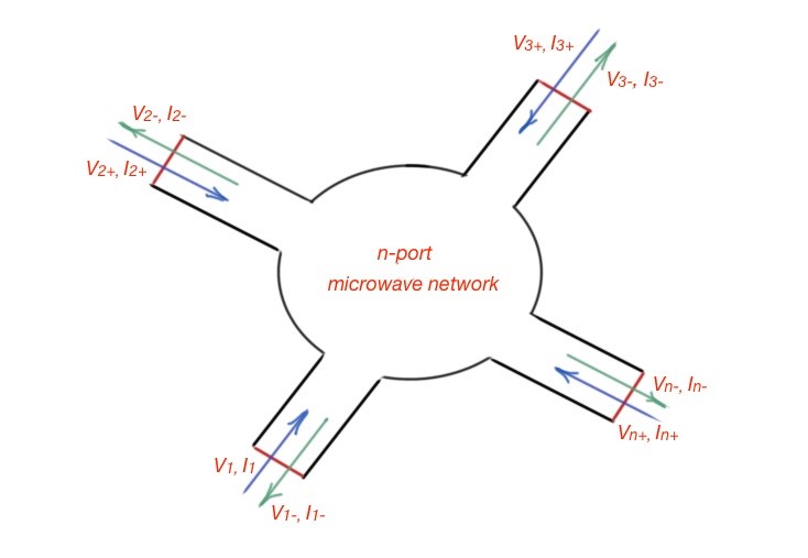 Figure 1. The N-port microwave network.
In the same way, the admittance matrix for the microwave system can be defined as: .
So the relationship between the admittance and impedance matrices are . An arbitrary reciprocal microwave system, which does not contain the active microwave components, or ferrites, is characterised with two independent sources of electromagnetic fields, so they will work using the reciprocal theorem: . The admittance and impedance matrices are symmetrical for reciprocal systems and imaginary for lossless networks.
When working with high frequencies it is good to do so with scattering matrices, but not with impedance or admittance matrices. The scattering matrix also describes the N-ports’ electromagnetic network. The difference between these two types of matrices are that the admittance and impedance matrices operate with the full values of voltages and currents, and scattering matrix operate with the ratios of incident and reflected wave characteristics.
Scattering matrix elements can be in most cases, measured with a vector network analyser. The scattering matrix can be represented the following way: .
The scattering matrix can be represented with the impedance matrix and characteristic impedances only if they are identical for all the network terminals.
For the reciprocal network the scattering matrix is symmetrical, and for the lossless microwave networks, the scattering matrix is unitary. The matrix is called unitary if the conjugated transpose matrix is equal to the same inversed matrix.
If all the ports of the microwave network are matched, then the reflection coefficient of the N-port is equal to the . The transmission coefficient from the M-port to N-port is equal to .
In case of losses of transmission waves at the microwave network, we can introduce power waves that can be determined in the following way: , here which is the reference impedance. From these statements we can also find total voltage, current and power: , and the total power . The reflection coefficient for the reflected power wave can be viewed as: .
The impedance, admittance and scattering matrices are used to describe the networks with multiple ports. However, usually microwave connections are cascaded into a system, which enables us to define the other type of useful calculation matrix – the ABCD matrix. This matrix is a relationship between the characteristic currents and voltages of every two-port connection between microwave networks. The handbooks for microwave systems describe the ABCD parameters of this matrix for any cascade connection of the networks.
The signal flow graph is the other technique for determining the microwave network parameters. Let’s consider the two-port network, depicted in Figure 2. Here we can see the incident wave with the amplitude , that goes through the network, and the transmitted wave with the amplitude . This wave will be partially reflected and re-enter the two-port network with the amplitude , part of this wave will got through the network port with the amplitude .
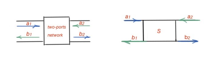 Figure 2. Two terminal microwave network with its scattering matrix representation. The blue waves are incident and transmitted, the green waves are reflected and transmitted back.
The Figure 3 shows decomposition rules for the waves through the microwave network.
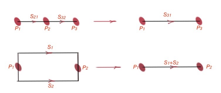
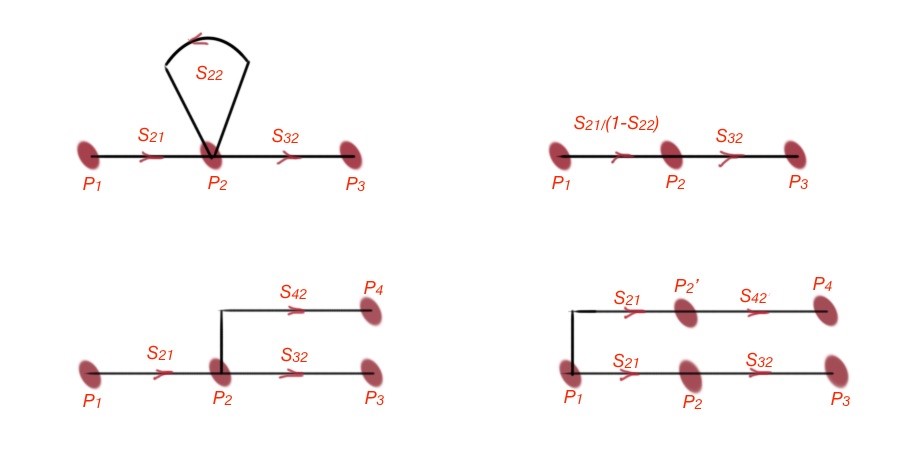 Figure 3. Decomposition rules for microwave networks. [1]
[1] «Microwave engineering”, 4th edition, David M.Pozer.