Smith Chart

The Smith Chart is shown in Figure 1. It is a very useful tool for solving the problems of RF engineers with regards to transmission lines. It was developed in 1939 by Phillip H. Smith, and despite of being developed so long ago, it is still in use and is the most famous and helpful tool among engineers.

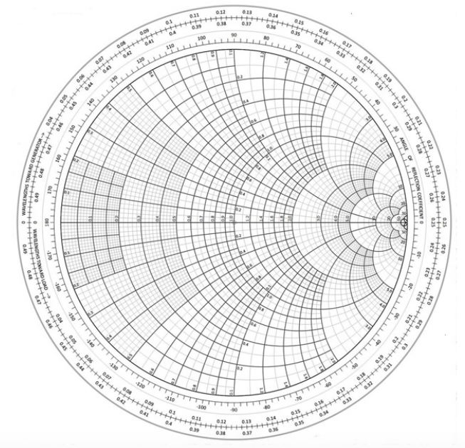
The Smith Chart is based on the polar system of the voltage reflection coefficient Г. The reflection coefficient is in the polar form $Г=\left|Г\right|e^{j\theta }$, where $\left|Г\right|$ is the reflection coefficient magnitude radius from the plot centre. And θ is the angle between the reflection coefficient vector and the chart horizontal diameter, -180<θ<180. A useful aim of the Smith Chart is that it can convert reflection coefficients to the normal impedances and reverse.

To do so, impedance or admittance circles should be depicted in the chart. Regarding the impedance, it is better to use normalised quantities $z=\frac{Z}{Z_0}$ , where  is an impedance, Z₀ is a lossless transmission line impedance. Let’s assume Z_L is a load impedance. So the reflection coefficient $Г=\frac{z_L–1}{z_L+1}=\left|Г\right|e^{j\theta }$, here $z_L=\frac{Z_L}{Z_0}$ , or $z_L=\frac{1+\left|Г\right|e^{j\theta }}{1+\left|Г\right|e^{j\theta }}$.

At the beginning of the RF and Microwave course we showed that all the quantities can be represented with their real and imaginary parts. So let’s represent the reflection coefficient and load resistance as complex values: $Г={Г}_r+j{Г}_i,z_L=r_L+j{x}_L.r_L+j{x}_L=\frac{1+{Г}_r+j{Г}_i}{1–{Г}_r–j{Г}_i}$ . Resolving the real and imaginary parts of impedance are: $r_L=\frac{1–{Г}_r^2–{Г}_i^2}{(1–{Г}_r{)}^2+{Г}_i^2},x_L=\frac{2{Г}_i}{(1–{Г}_r{)}^2+{Г}_i^2}$ . These equations can be rearranged to represent the resistance and reactance circles on the Smith Chart: $\frac{{Г}_r–r_L}{(1+r_L{)}^2}+{Г}_i^2=\frac{1}{(1+r_L{)}^2},({Г}_r–1{)}^2+({Г}_i–\frac{1}{x_L}{)}^2=(\frac{1}{x_L}{)}^2$ . We can see that all the reactance circles lie on the vertical line ${Г}_r=1$ , and all the resistance circles lie on the horizontal line ${Г}_i=0$ . The Smith Chart can be very useful to resolve graphically the transmission line equation, so the input impedance of the transmission line is: $Z_{i}n=Z_0 \frac{1+Гe^{–2j\beta l}}{1–Гe^{(–2j\beta l}}$ , where $Г$ is the reflection coefficient of the transmission line and l is the length of the transmission line. This result is similar to the normalised impedance, the difference is only in the rotating angle of the plot. The rotation angles of the plot are related to the wavelength of the transmission line.

The Smith Chart can also be used for resolving admittance of the transmission line, as admittance and impedance are related to each other. The Smith Chart usually has both impedance and admittance scales. Below are examples of how to use the Smith Chart with real components.

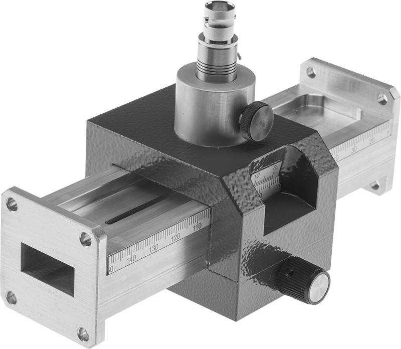
A slotted line, used in the RF measurements, consists of a probe (waveguide or coaxial line), allowing the sampling of the electric field amplitude of the standing wave of the terminated line. This allows us to determine the load impedance, and as the load impedance is the complex number, then the slotted line should measure two quantities.

Figure 2 depicts the usual slotted line. Let’s assume that we measured the SWR and $l_{min}$, the distance to the first voltage minimum across the terminated line. So, the reflection coefficient of the transmission line is $\left|Г\right|=\frac{SWR–1}{SWR+1}$ , where the SWR is the standing wave ratio. The voltage minimum should occur when $e^{(\theta –2\beta l)}=–1, so \theta =\pi –2\beta l_{min}$ . The voltage minimum repeats every half wavelength. And knowing the reflection coefficient we can find the load impedance.

(Microwave Engineering, 4th edition, David M. Pozar).

Quarter-wave impedance transformer