Electromechanics – main terms

Elelctromagnetic forces are used to produce mechanical effects that are considered in terms of  electromechanics. The applications of electromechanics are fairly wide like in electric motors and electromagnets. 

Magnets are very important in the field of elelctromechanics. Magnets can affect conductors, insulators and semiconductors without physical contact. As we know magnets are characterised by magnetic field, measured by the magnetic flux density B, Ts and magnetic field intensity H, A/m.

If the charge q is moving in the magnetic field with the speed v then there will be a force acting on the conductor perpendicular to the conductor and the magnetic field. The force magnitude is $f=q\left[v,B\right]$, $N$. If the conductor speed (or charge) is directed with some angle to the field, then the force magnitude is $f=qvB\sin \theta$, where $\theta$ is the angle between the charge speed and the field.

Another characteristic of the magnetic field is the magnetic flux $\varphi =\int BdA$ – that is integral to the magnetic flux density $B$ over the cross-sectional area $A$. The magnetic flux $\varphi$, is measured in Webers (Wb).

Faraday’s Law states that the magnetic field B through the surface A, bounded by the conductor, induces the potential difference and the current through the conductor. If the magnetic flux ϕ varies in time, it can induce the electro-motive force $EMF \epsilon =–\frac{\partial \varphi }{\partial t}$.

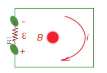
Let’s consider a single-loop coil, closed by the resistor R. Let’s suppose that the magnetic field B flows through this coil, as shown in Figure 1. Then the current  will flow through this coil, creating the field in the opposite direction to the magnetic field B. This effect is known as Lenz Law. By the right-hand rule, there will be a current provoked by the generated field, moving clock-wise. And the voltage across the resistor will be negative.

In practice the voltage magnitude can be increased by increasing the quantity of coils (the bigger quantity of coils, the bigger surface the magnetic flux goes through). So for N coils  $\epsilon =N\frac{\partial \varphi }{\partial t}$.

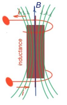
On the figure below you can see the N-turns coil, linking the flux B, and as the coils are close to each other, we can then suppose the term of the flux linkage is $\lambda =N\varphi and \epsilon =\frac{\partial \lambda }{\partial t}$.

So, how can we generally change the magnetic flux and provoke the electro-motive force ɛ? We can physically move the magnet in the vicinity of the coil, to provoke the electro-motive force. Or we can produce the magnetic field by electric current and just change the electric current. The voltages, generated by the moving in time voltages, are called transformer voltages. This effect is used in some electromechanical devices.

From the general course of electromagnetism the relationship between the linkage flux and current is $\lambda =Li$. So the current, changing in time, provokes the transformer voltage $v=L\frac{di}{dt}$.

The L parameter is self-inductance. If these two circuits are close to each other, it will lead to the effect of magnetic coupling, when the second circuit will also experience the provoked magnetic flux by the current of first circuit. This effect lies in the base of the transformers.

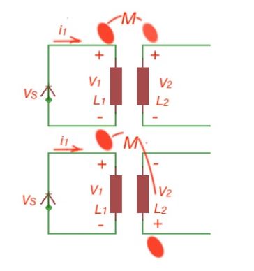
Let’s consider two coils. One of them is connected to the current source $i_1$, The inductance $L_1$ generates voltage $v_1$. The second coil $L_2$ is not connected to the current source, but the excited magnetic field of the first coil induces the voltage in a second coil $L_2$. This magnetic coupling happens because the proximity of two coils and is called the mutual inductance, which is characterised by the formula $v_2=M_2\frac{d{i}_1}{dt}$.

The voltage polarity in the coils are depicted below. In real electromagnetic circuits self-inductance is not always constant. In practice the relationship between linkage flux and the current is not linear at all. And it is easier to operate in terms of energy in the magnetic circuit calculations.

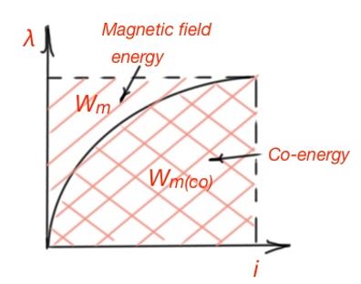
Let’s consider the relationship between flux linkage $\lambda$ and the current . Energy stored in the magnetic field of the magnetic system is $W_m=\int P_{i}dt=\int \epsilon idt$. The induced emf at the magnetic system is $\epsilon =N\frac{d\varphi }{dt}$.

And the energy is $W_m=\int \epsilon idt=N\int \frac{d\varphi }{dt}idt=N\int id\varphi =\int id\lambda$.

This energy corresponds to the area above the curve. The area under the curve is called co-energy:

$W_m^{co}=i\lambda –W_m$

Another important relationship for electromechanical devices is the Ampere Law, which states that the integral of the magnetic field H, closed by the loop l, is equal to the current carried by the loop$\oint Hdl=\sum _{}i$. Another important term is magnetomotive force (MMF) that is described by the formula $F=Ni$.

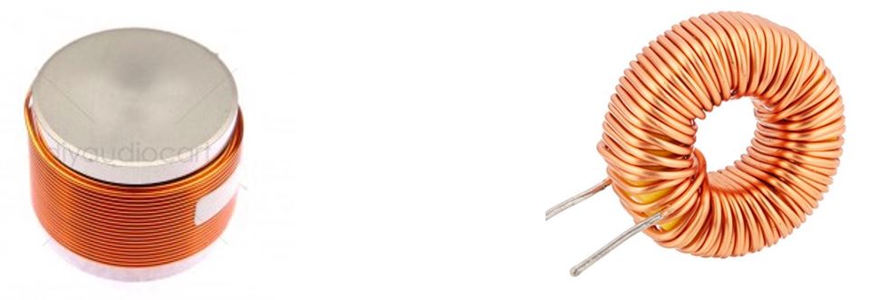
In terms of applications, when the coil encloses the magnetic material, the greater magnetic flux is generated. The most frequent ferromagnetic materials are steel, iron and ferrites. The coiling of the magnetic material helps to keep the magnetic field with considered shape close to the magnetic material. The magnetic field in the area of the coil is depicted in Figure 5. The magnetic flux for the most practical inductors are:

$B=\frac{\mu Ni}{l}(for the iron–core coil), B=\frac{\mu Ni}{2\pi r_2}(for torodial coil)$

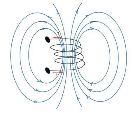
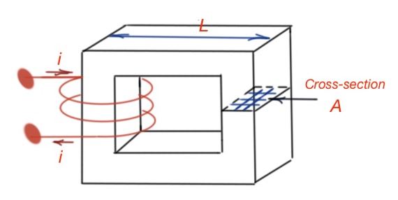
Figure below shows the structure of a simple transformer. Let’s make the assumption that there is a mean path for a magnetic flux to exist, and that it corresponds to the mean magnetic flux density. The mean flux density is constant over the cross-sectional area of the magnetic structure $B=\frac{\varphi }{A}$.

The cross-sectional area A is assumed to be perpendicular to the magnetic flux lines.

The field intensity is $H=\frac{B}{\mu }=\frac{\varphi }{\mu A}$. MMF for this magnetic structure is $F=H^{*}I=\frac{\varphi I}{\mu A}$. Parameter $R=\frac{I}{\mu A}$is called reluctance. The relationship between the inductance of the magnetic material and the reluctance is $L=\frac{N^2}{R}$.

It does mean that for an N-turn coil winding the magnetic core, with current $i$, it’s the MMF $F$ that generates the magnetic field flux $\varphi$, that is mostly concentrated within the core and is uniform in its cross-sectional area.

Let’s consider the magnetic structure and its equivalent circuit. We can represent the magnetic structure with an equivalent circuit with four legs, and MMF as a source. Two paths here have the mean path $I_1$ with the cross-sectional area $A_1=d_1\omega$, and two legs with the mean path $I_2$ with cross sectional area $A_2=d_2\omega$. Then the reluctance of the magnetic core is $R_{total}=\frac{1}{{\mu }_0{\mu }_{R}S}(l_1+l_2+l_3+l_4+l_5)+\frac{\delta }{{\mu }_0{S}_{\delta }}$.

 

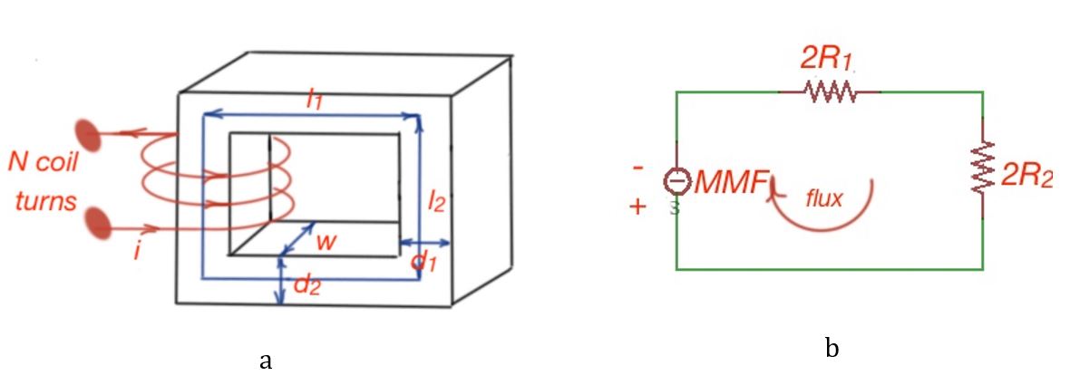
When the square of the gap area is bigger than the cross-section of the magnetic material, this phenomena is called fringing and happens because the magnetic field is spread more in the air gap. After the theoretical part we will consider some examples of real magnetic structures to calculate.

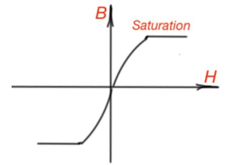
From the previous chapters of the electromagnetism course we know that μ permeability of magnetic material is not a linear function of flux density B and field intensity H, but has the following form .

The idea of this non-linear relationship between flux density and field intensity is grounded on the following basis. The big importance here is based on the spin of the electron. In most materials except ferromagnets, spin doesn’t constitute a big role.

Ferromagnets demonstrates the domain structure of the material, and the magnet field makes the domains oriented to an exact direction. At a certain moment all the domains will be oriented and any further magnetic field impacts won’t make sense.

This moment is called saturation. There are two reasons why the relationship of B and H are not linear – the eddy currents and hysteresis loop. The eddy currents are the closed electrical current loops that are induced by the time the varying magnetic fields are caused by Faraday’s Law of induction. The hysteresis loop happens when the conductor occurs in the external magnetic field, and its domains become aligned.

Transformers and their types