Transient processes in linear circuits

Transient processes in electrical circuits are the processes of transition from one work regime to another, that differ with parameters. Transient processes are caused by the commutation in the circuit (closing and opening of the circuit with electrical switch).

So a transient process is the process of energy state transition of the circuit from prior-commutation state to after-commutation state. Transient processes are very short, usually about a ten-hundredth of second. However, it is important to know the transient process length, the how the signal changes between the circuits states.

Let’s consider the transient process as depicted on the figure below. It can be described with the differential equation $L\frac{di}{dt}+Ri=E$. The solution for this equation is the function  $i\left(t\right)=\frac{E}{R}–\frac{E}{R}{e}^{–\frac{R}{L}t}$.

This solution consist of two parts – a general and proprietary solution. The proprietary solution of a differential equation is the forced current component, general solution – and is the free current component. So the general solution is $i=i_{free}+i_{pr}$.

The proprietary current or voltage component has the same frequency and waveform as the EMF in the circuit. If the EMF of the circuit is constant, then current through the capacitor is zero, and voltage through the inductor is zero. We should remember this statement along the whole course. The free component of the current or voltage in the linear circuit has an exponential form and usually decaying.

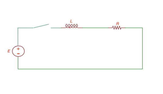
 The example of the circuit, performing the transient process.

The total current or voltage is the current or voltage going through the circuit during the transient process, and can be measured and seen on the measurement equipment. The proprietary and free components are playing a second role here.

Task 1. Show that the current through the inductor and voltage through the capacitor can’t change intermittently.

The procedure for transient process analysis.
• To set up the positive directions of currents and voltages in the circuit;
• Determine currents and voltages before commutation ;
• Characteristic equation resolution;
• Obtaining currents and voltages as functions of time.

Let’s consider commutation rules. The first rule of commutation states that current through the inductor before the transient process is equal to the current through this inductor after commutation $i_L(t=0–)=i_L(t=0+)$. The second rule of commutation states that voltage of the capacitor before the transient process is equal to the voltage of this capacitor after commutation $u_C(t=0–)=u_C(t=0+)$.

The start currents and voltages are those when $t=0$. Different components of the circuit may have different values after the transient process, except the ones, that work with commutation rules. So for different components we can also have prior-commutation values and after-commutation values – the values before and after transient process.

The after-commutation process can be described with the Kirchhoff’s laws. Here currents through the inductances and voltages through the capacitors are independent start values, and the rest of the circuit parameters are dependent start values. If there are zero currents and voltages through the circuit before commutation, then the start values are zero, otherwise they are non-zero.

So how do we resolve Kirchhoff’s equations for circuit currents after the transient process? Choose the positive current directions, write down Kirchhoff’s equations for all circuit branches (for the total current).

After that we have to erase the voltage sources in the circuit and write down Kirchhoff’s equations for free currents. As a result we will get the differential equation. As we know from above the free current changes exponentially, and the solution of the differential equation is an exponential function $e_{free}=A{e}^{bt}$.

So $\frac{d{e}_{free}}{dt}=b{i}_{free}$. Here ${\int }_{}^{}{i}_{free}dt=\frac{i_{free}}{b}$. These expressions give us the voltage of the capacitor $\frac{i_{free}}{Cb}$. Let’s consider the example circuit in Figure 2. The Kirchhoff equations for free currents here are: $i_1+i_2+i_3=0, (Lb+R)i_1+i_{2}r=0, i_{2}r–\frac{i_3}{Cb}=0$

These equations are algebraic, not differential, which simplifies the process of current calculation. These equations can be resolved with the determinant method, known from linear algebra. Let’s define the free currents in the following way: $i_1=\frac{{∆}_1}{∆}, i_2=\frac{{∆}_2}{∆}, i_3=\frac{{∆}_3}{∆}$, here

$∆=\left|\begin{array}{ccc}1& –1& –1\\ Lb+R& r& 0\\ 0& r& –\frac{1}{Cb}\end{array}\right|$, ${∆}_1=\left|\begin{array}{ccc}0& –1& –1\\ 0& r& 0\\ 0& r& –\frac{1}{Cb}\end{array}\right|$, ${∆}_2=\left|\begin{array}{ccc}1& 0& –1\\ Lb+R& 0& 0\\ 0& 0& –\frac{1}{Cb}\end{array}\right|$, ${∆}_3=\left|\begin{array}{ccc}1& –1& 0\\ Lb+R& r& 0\\ 0& r& 0\end{array}\right|$.

It means that all the free currents $i_1=0, i_2=0, i_3=0$. However, free currents can be different from zero, if $∆=0$. This equation is a characteristic equation, that helps us to determine the b parameter.

Another way to obtain the b parameter is to create the input internal resistance of the two terminal with the AC $Z\left(\omega \right)$ , to replace ω with b and resolve the characteristic equation $Z\left(b\right)=0$.

The relation between these two methods is that the conductance and resistance of the circuit branches can be represented through the operators mentioned above. The solution of the characteristic equation may have a number of roots – all should be counted and the total current value will be a sum of these roots of the characteristic equation.

The characteristic equation order can be determined by the quantity of independent input parameters of the after-commutation circuit. For the simple analysis of the circuit the series connection of inductances and capacitances should be replaced with equivalent inductances and capacitances.

The types of the roots of characteristic equation tells us about the type of signal. Resulting signals can vary depending on type and quantity of the roots – they can be exponential (so the resulting signal is exponential), they can be real, and they can be complex, complex-coupled – and all these variations can determine different resulting signals.

Doing the switching-off in the circuit with huge values of inductances can be dangerous, because of the overdrives generated on the different circuit parts. These voltages can be much bigger than the voltages of the stable circuit, that involves risks for the circuit.

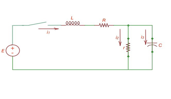
The example of a circuit performing the transient process.

There are a few more methods of resolving characteristic equations – operator method, integral Duamel method, and some others you can read about in supporting literature. However, operator method is very useful and will be described further.